Constraint Satisfaction Problems (CSP)

Definition of CSP

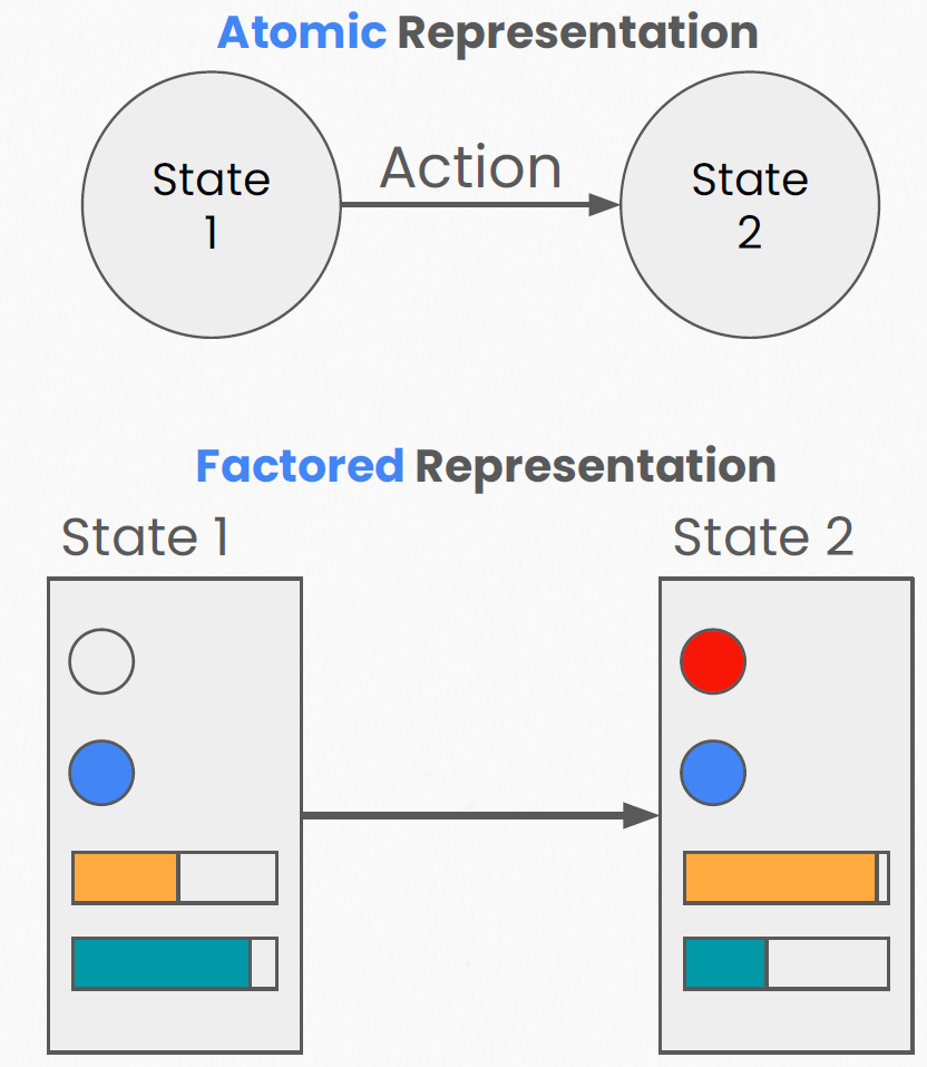
As shown in the figure below, in traditional search we do not examine the internal structure of a state — this is known as an atomic representation. In the CSP approach, we use a factored representation, where a state is decomposed into a set of variables and their values.

A CSP is defined by:

• Variables (\(X\)): The set of objects that need to be assigned values (\(X_1, ..., X_n\)).
  • Example: each region in a map-coloring problem.
• Domains (\(D\)): The set of possible values for each variable (\(D_i\)).
  • Example: {Red, Green, Blue}.
• Constraints (\(C\)): Rules that restrict the values variables can take (\(C_m\)).
  • Example: adjacent regions must not share the same color (\(X_1 \neq X_2\)).
• Goal: Find an assignment that satisfies:
  1. Completeness: Every variable is assigned a value.
  2. Consistency: No constraint is violated.

Backtracking Search

Backtracking Search is the standard algorithm for solving CSPs. It is essentially a depth-first search (DFS) optimized for CSPs.

Workflow:

1. Select one variable at a time to assign (rather than generating an entirely new state).
2. Check whether the assignment satisfies the current constraints.
3. If it does: recursively continue assigning the next variable.
4. If it does not: abandon the current branch, backtrack to the previous step, and try the next value in the domain.

Core idea: "Fail fast" — as soon as a dead end is detected, backtrack immediately instead of waiting until the end to discover the failure.

Constraint Propagation

Constraint Propagation is a technique used to accelerate backtracking search.

As the name suggests, we can leverage constraints to deduce which values are impossible early on, thereby shrinking the domains of variables.

Common methods include:

• Forward Checking: After assigning a value to variable \(X\), immediately inspect all unassigned variables connected to \(X\) and remove any values from their domains that conflict with \(X\)'s assignment. If any variable's domain becomes empty, backtrack immediately.
• Arc Consistency (AC-3): More powerful than forward checking. Before or during assignment, it propagates constraints through a chain reaction, ensuring that every arc (edge) in the constraint graph is consistent. This allows infeasible situations to be detected even earlier.

Variable Ordering Heuristics

The efficiency of backtracking search depends critically on the order in which variables are selected for assignment — choosing the right variable first can dramatically reduce the search space.

Minimum Remaining Values (MRV)

The Minimum Remaining Values (MRV) heuristic, also known as the "most constrained variable" or "fail-first" heuristic, follows this strategy:

Select the variable with the fewest remaining legal values in its domain.

The intuition is straightforward: if a variable has only 1 legal value left, it must take that value; if one variable has 2 remaining values while another has 10, addressing the former first will expose contradictions sooner.

Formally, at each step of backtracking search, we select:

\[ X^* = \arg\min_{X_i \in \text{unassigned}} |D_i| \]

where \(D_i\) is the current effective domain of variable \(X_i\) (the set of remaining values after constraint propagation).

Why MRV Works

MRV is called "fail-first" because it prioritizes the variable most likely to cause failure. While this may seem counterintuitive, it triggers backtracking early, avoiding wasted effort on branches that are doomed to fail. Empirically, MRV significantly reduces the number of nodes explored in most CSP problems.

Degree Heuristic

The Degree Heuristic is used as a tiebreaker when MRV produces a tie. Its strategy is:

Select the variable that is involved in the most constraints with other unassigned variables.

Formally, the "degree" of variable \(X_i\) is defined as the number of constraints between \(X_i\) and other unassigned variables. The degree heuristic selects the variable with the highest degree:

\[ X^* = \arg\max_{X_i \in \text{unassigned}} \text{deg}(X_i) \]

The intuition is that the variable with the highest degree constrains the most other variables; assigning it first maximally shrinks the domains of subsequent variables.

In a map-coloring problem, the degree heuristic would prioritize the region adjacent to the most uncolored neighbors.

Value Ordering

Variable ordering determines which variable to assign next, while value ordering determines which value to try first.

Least Constraining Value (LCV)

The Least Constraining Value (LCV) heuristic follows this strategy:

Try the value that rules out the fewest choices for neighboring unassigned variables.

Specifically, for the currently selected variable \(X_i\), we evaluate each value \(v \in D_i\) by counting how many values it would eliminate from the domains of neighboring variables. We choose the value that eliminates the fewest:

\[ v^* = \arg\min_{v \in D_i} \sum_{X_j \in \text{neighbors}(X_i)} |\text{eliminated}(X_j, v)| \]

where \(\text{eliminated}(X_j, v)\) denotes the number of values removed from \(X_j\)'s domain as a consequence of setting \(X_i = v\).

Variable Ordering vs. Value Ordering: Opposing Philosophies

Notice that MRV and LCV pull in opposite directions:

• MRV (variable ordering): Fail-first — tackle the hardest variable first to detect dead ends early.
• LCV (value ordering): Succeed-first — try the most promising value first to avoid dead ends.

The two work best in combination: select the most constrained variable (MRV), then try the least constraining value (LCV).

Local Search for CSPs

In addition to backtracking search, we can solve CSPs using local search methods. Local search starts from a complete but potentially inconsistent assignment and iteratively modifies variable values to reduce the number of constraint violations.

Min-Conflicts Algorithm

Min-Conflicts is the most classical local search method for CSPs:

function MIN-CONFLICTS(csp, max_steps):
    current ← randomly assign an initial value to every variable
    for i = 1 to max_steps:
        if current satisfies all constraints:
            return current
        var ← randomly select a variable that is in conflict
        value ← choose the value that minimizes the number of conflicts for var
        set var = value
    return failure

The core steps:

1. Random initialization: Assign a random value to every variable (regardless of constraint satisfaction).
2. Select a conflicted variable: Randomly pick a variable whose current value violates at least one constraint.
3. Minimize conflicts: Change that variable's value to the one that minimizes the total number of conflicts (break ties randomly).
4. Repeat until a solution is found or the maximum number of iterations is reached.

Efficiency of Min-Conflicts

A remarkable property of Min-Conflicts is that for many CSP problems (including the \(n\)-queens problem), it finds a solution in roughly constant time, independent of problem size. For example, the 1-million-queens problem can be solved in approximately 50 steps on average. This is because most random initial assignments are already close to a solution and require only a small number of local adjustments to converge.

Limitations of Local Search

The main drawback of local search is the tendency to get stuck in local minima — states where no single-variable change reduces the number of conflicts, yet the current assignment is not a global solution. Common strategies to mitigate this include:

• Random Restart: When stuck in a local minimum, reinitialize randomly.
• Random Walk: With some probability, choose a random value (instead of the conflict-minimizing value) to escape local minima.
• Simulated Annealing: Accept worse solutions with a probability that decreases over time.
• Tabu Search: Maintain a "tabu list" to prevent revisiting recent assignments.

CSP as Optimization

So far, the CSPs we have discussed involve hard constraints: a constraint is either satisfied or violated. In the real world, however, many problems involve soft constraints and preferences.

Soft Constraints and Weighted CSP

A Weighted CSP or Constraint Optimization Problem (COP) assigns a weight or cost to each constraint:

• Hard constraints: Must be satisfied; violation renders the solution invalid (weight = \(\infty\)).
• Soft constraints: Violation incurs a cost but does not invalidate the solution.

The objective shifts from "find an assignment satisfying all constraints" to "find an assignment that minimizes total cost":

\[ \min_{\text{assignment}} \sum_{C_m \in \text{soft constraints}} w_m \cdot \mathbb{1}[\text{violated}(C_m)] \]

where \(w_m\) is the weight of constraint \(C_m\) and \(\mathbb{1}[\text{violated}(C_m)]\) equals 1 when the constraint is violated.

In a more general form, each soft constraint defines a cost function \(f_m\), and the total cost of an assignment is:

\[ \min_{\text{assignment}} \sum_{C_m} f_m(\text{assignment}) \]

Common Optimization Methods

Weighted CSPs can be solved using:

• Branch and Bound: Maintain an upper bound on the cost of the current best solution during backtracking, and prune branches whose cost already exceeds this bound.
• Local Search: Use a weighted variant of Min-Conflicts, selecting values that minimize weighted conflict cost.
• Integer Linear Programming (ILP): Formulate the CSP as a mathematical programming problem and solve it with mature solvers.

Real-World CSP Applications

The CSP framework is remarkably general and can model a wide range of practical problems.

Course Scheduling

University course scheduling is a classic CSP problem:

• Variables: The time slot and classroom for each course.
• Domains: All available time slots and classrooms.
• Constraints: * The same professor cannot teach two courses at the same time (hard constraint). * The same classroom cannot host two courses simultaneously (hard constraint). * Classroom capacity must accommodate enrollment (hard constraint). * Minimize scheduling conflicts for students enrolled in multiple courses (soft constraint / preference). * Instructor time-slot preferences (soft constraint / preference).

Sudoku

Sudoku is a particularly clean CSP instance:

• Variables: Each empty cell \(X_{ij}\) in the \(9 \times 9\) grid.
• Domains: \(D_{ij} = \{1, 2, ..., 9\}\).
• Constraints: * All digits in each row must be distinct (All-Different constraint). * All digits in each column must be distinct. * All digits in each \(3 \times 3\) box must be distinct.

Sudoku is well suited to arc consistency + backtracking search + MRV. In fact, for most Sudoku puzzles, arc consistency (AC-3) alone resolves the majority of cells, and only a small amount of backtracking is needed to complete the rest.

Other Applications

The CSP framework is also widely used in:

• Map coloring: Assign colors to regions of a map such that no two adjacent regions share the same color (the classic graph coloring problem).
• Resource allocation: Distribute limited resources among multiple tasks subject to various constraints.
• Circuit design: Layout and routing of electronic components.
• Natural language processing: Constraint propagation in part-of-speech tagging and syntactic parsing.
• Computer vision: Label consistency constraints in scene labeling and image segmentation.

---

评论