Simulation World Building & Physics Rules
Robot simulation is not just "drop a few assets into a simulator." A world that is actually usable for training, evaluation, and deployment transfer must answer three questions at the same time:
- How is the world organized?
- What physical rules does it follow?
- How is it validated, randomized, and aligned to Sim2Real?
This note is not about individual assets. It is about how assets become a world. It sits after Simulation Assets, below Simulation Platforms, and upstream of Sim2Real: the asset note tells you what the parts are, while this note explains how those parts become a runnable, trainable, and transferable universe.
1. World Building Overview
1.1 What a "simulation world" actually is
In embodied AI, a world is usually not just a 3D scene file. It is a composition of several layers:
At minimum, a world must define:
- what entities exist
- how they are organized
- how they move and contact
- when tasks start and end
- what the policy can observe and control
1.2 World, scene, task, and episode
| Concept | Meaning | Typical example |
|---|---|---|
| World | top-level container for scene, rules, and task interface | KitchenPickWorld |
| Scene | static or semi-static spatial layout | countertop, warehouse aisle |
| Task | goal definition plus success criterion | Pick red mug |
| Episode | one rollout from reset to done | one trial |
| Domain | parameter distribution and randomization space | lighting, friction, latency |
| Benchmark | standardized task set plus evaluation protocol | LIBERO, RLBench, SIMPLER |
1.3 What makes a world "good"
| Dimension | Requirement |
|---|---|
| correctness | consistent physics, frames, sensors, and task logic |
| stability | long rollouts do not explode |
| controllability | reset, sampling, and randomization are configurable |
| reproducibility | fixed seeds reproduce behavior |
| extensibility | new assets, sensors, and tasks can be added cleanly |
| transferability | the world is useful for Sim2Real |
1.4 World building from the simulator viewpoint
graph TD
    A[Simulation platform] --> B[Asset loading]
    B --> C[World hierarchy]
    C --> D[Physics configuration]
    D --> E[Sensors and observations]
    E --> F[Task logic and rewards]
    F --> G[Reset / randomization / evaluation]

    style A fill:#e3f2fd
    style B fill:#fff3e0
    style C fill:#e8f5e9
    style D fill:#fce4ec
    style E fill:#f3e5f5
    style F fill:#ede7f6
    style G fill:#fff8e1
1.5 Why the world layer is underestimated
Algorithm work often silently assumes that:
- reset is always clean
- contacts are always stable
- cameras always point in the right direction
- parallel environments behave consistently
In real projects, the world layer has to guarantee all of that. Many "algorithm differences" are actually world-layer bias.
2. World Organization and Hierarchy
2.1 A generic hierarchy
graph TD
    W[World] --> S[Scene]
    S --> E[Entity]
    E --> C[Component]
    E --> T[Task Hooks]
    C --> P[Physics]
    C --> R[Render]
    C --> N[Sensor]
    T --> Reset[Reset Logic]
    T --> Reward[Reward / Success Logic]
2.2 Common organizational styles
| Style | Representative systems | Characteristics |
|---|---|---|
| tree-structured scene graph | USD, Smallville | clear hierarchy, strong composition |
| recursive worldbody | MuJoCo | tight coupling between physics and hierarchy |
| ECS / component-based | Unity, parts of game-engine-style simulators | decoupled and modular |
| config-driven world + task | Isaac Lab, ManiSkill | close to training workflows |
2.3 Lesson from Smallville
In Virtual World Simulation Engines, the Smallville example looks like social simulation, not robotics. But it demonstrates an important engineering idea: a world is not just an image or a mesh. It is a semantic tree.
World
|- House
|  |- Kitchen
|  |  |- Table
|  |  \- Cup
|  \- Bedroom
\- Cafe
That matters in robot simulation because a semantic tree helps with:
- local transforms
- partial loading
- semantic inheritance
- localized resets
2.4 USD scene graphs
USD is attractive for large worlds because it supports:
- references
- instancing
- layered composition
- transform inheritance
That enables a world assembled from:
- base architecture layer
- furniture layout layer
- robot layer
- lighting layer
- task-object layer
- randomization override layer
2.5 SDF worlds
SDF is closer to a complete world definition:
- world
- model
- link
- joint
- light
- physics
- plugin
For Gazebo, world building is not just placing geometry. It is also putting engine settings, sensors, and bridge behavior into a unified description.
2.6 MuJoCo worldbody
MuJoCo emphasizes:
- recursive body hierarchy
- tight coupling of geoms and joints
- a unified physical view of contacts, actuators, and sensors
It is less naturally suited than USD for large collaborative asset libraries, but it is extremely efficient for research-driven world design.
2.7 What should be an entity vs a component
| Object | Better modeling choice |
|---|---|
| robot | independent entity |
| drawer | independent entity with internal articulated subparts |
| light | scene component or standalone entity |
| sensor rig | usually attached to an entity but managed as a reusable component |
| success criterion | world/task-layer logic, not an entity |
2.8 Hierarchy checklist
| Item | Question |
|---|---|
| root frame | does every object have a clear root frame? |
| naming | are scene-graph names stable enough for code and datasets? |
| composition | can new assets be inserted without rewriting the tree? |
| local reset | can task objects be reset independently? |
| semantics | can semantic labels be recovered from hierarchy? |
3. Coordinate Frames and Time Systems
3.1 Why frame bugs are more common than physics bugs
One of the most common low-level causes of training failure is frame mismatch:
- wrong camera frame
- wrong end-effector frame
- object pose expressed in the wrong reference
- reward computed in world frame while actions are applied in robot frame
3.2 Common frames
| Frame | Role |
|---|---|
world |
global reference |
map |
long-horizon localization frame |
base_link |
robot base |
tool0 / tcp |
end-effector tool frame |
camera_frame |
physical camera body |
camera_optical_frame |
optical projection convention |
object_frame |
object-local reference |
3.3 Transform chains
The core transform relation is:
This shows up everywhere in world building:
- robot base to camera
- world to object
- table to mug
- mug to grasp pose
graph LR
    W[World] --> B[Robot base]
    B --> T[Tool]
    W --> O[Object]
    T --> G[Grasp pose]
    O --> G
3.4 Preferred frames by task
| Task | Preferred reference | Why |
|---|---|---|
| end-effector pose control | robot base / tool frame | more stable control semantics |
| object grasping | object frame + tool frame | easier grasp specification |
| navigation | map / world | clearer planning geometry |
| multi-camera fusion | world + camera rig | easier extrinsic consistency |
3.5 Time systems
Worlds need time systems as much as spatial frames:
| Concept | Meaning |
|---|---|
| simulation time | simulator clock |
| wall-clock time | actual elapsed runtime |
| fixed step | physics step size |
| render step | rendering update interval |
| sensor step | sensor refresh interval |
| control step | controller output interval |
3.6 Typical time relation
Let:
- physics step be \(\Delta t_p\)
- control step be \(\Delta t_c\)
- sensor step be \(\Delta t_s\)
- render step be \(\Delta t_r\)
Then a typical requirement is:
Otherwise control may run faster than state updates, or sensors may become misaligned with world state.
3.7 Real-time factor
The real-time factor is:
RTF > 1: simulation runs faster than real timeRTF = 1: real-time simulationRTF < 1: simulation is slower than real time
Training wants RTF as high as possible. Human-in-the-loop debugging and digital twins often care more about staying near 1.
3.8 Debugging frames and timing
| Problem | Typical debug method |
|---|---|
| frame mismatch | TF visualization, explicit axis drawing, manual pose sanity checks |
| time desynchronization | inspect timestamps and lag |
| wrong optical frame | verify projection direction |
| render / physics mismatch | disable rendering and observe whether the bug remains |
4. Rigid-Body Dynamics Basics
4.1 Scope of this section
This section does not re-derive dynamics from first principles. For that, see Dynamics. Here the focus is how a simulator closes the minimum dynamics loop needed for a useful world.
4.2 Minimal rigid-body state
A rigid body is typically represented by:
- position \(\mathbf{x}\)
- orientation \(\mathbf{R}\) or quaternion \(\mathbf{q}\)
- linear velocity \(\mathbf{v}\)
- angular velocity \(\boldsymbol{\omega}\)
4.3 Core equations
For translation:
For rotation:
At the world-authoring level, that means at minimum you must supply:
- mass
- inertia
- external forces, including gravity
- constraints and contacts
4.4 Gravity is not the only force
Common force sources at world level include:
- gravity
- contact forces
- actuator outputs
- springs and dampers
- wind / fluid approximations
- injected perturbations for robustness testing
4.5 How asset parameters enter dynamics
| Asset field | Dynamics effect |
|---|---|
mass |
governs translational response |
inertia |
governs rotational response |
center_of_mass |
changes balance and attitude behavior |
joint damping |
dissipates velocity |
friction |
constrains tangential contact motion |
stiffness |
sets elastic constraint strength |
4.6 Free bodies and constrained bodies
| Object type | Character |
|---|---|
| free body | 6-DoF body moving freely |
| fixed body | rigidly attached to the world |
| joint-constrained body | motion restricted by joint type |
| contact-constrained body | motion additionally restricted by environment contact |
4.7 Energy view
Many "mysterious oscillations" are easier to understand in energy terms:
- too much drive energy injected
- not enough damping
- contacts solved too rigidly
- integrator error injecting artificial energy
4.8 How rigid-body dynamics appears in world templates
| World template | Most critical rigid-body issue |
|---|---|
| tabletop grasping | does the target object rest stably? |
| drawer manipulation | joint-contact coupling |
| insertion / assembly | precise contact under tight tolerances |
| quadruped terrain | foot contacts and base inertia |
| humanoid carrying | large payloads and whole-body stability |
5. Contact and Collision Rules
5.1 Why contact is the hardest part of world building
The largest gap between "the world runs" and "the world is trustworthy" is often contact.
If objects never touch, many things stay easy:
- rigid-body integration
- joint constraints
- visual observation
But once the task includes:
- grasping
- insertion
- stacking
- locomotion
- pushing and friction
contact becomes the system core.
5.2 Broad phase and narrow phase
flowchart LR
    A[All geometry] --> B[Broad phase<br/>discard obviously non-contact pairs]
    B --> C[Narrow phase<br/>compute actual contact points and penetration]
    C --> D[Constraint / Contact solver]
Broad phase tries to:
- shrink candidate pairs quickly
- avoid expensive exact tests
Narrow phase typically outputs:
- contact points
- normals
- penetration depth
- contact patches
5.3 Penetration and constraints
Contact is usually modeled as a constraint problem. Ideally, the normal gap should satisfy:
where \(\phi(\mathbf{x})\) is the gap function. If \(\phi < 0\), bodies are interpenetrating.
5.4 Friction cones
Tangential contact force is often bounded by:
where:
- \(\mathbf{f}_t\) is tangential friction force
- \(f_n\) is normal force
- \(\mu\) is the friction coefficient
For grasping, locomotion, and pushing tasks, friction modeling directly changes learnability.
5.5 Restitution and bounce
Restitution controls how much normal velocity is preserved after collision:
| Restitution regime | Typical behavior |
|---|---|
| close to 0 | highly inelastic, little bounce |
| intermediate | partial bounce |
| close to 1 | highly elastic |
High restitution often makes training unnecessarily noisy unless it is task-relevant.
5.6 Contact offset and rest offset
Many engines expose parameters such as:
contact offsetrest offset- penetration tolerance
- solver stabilization thresholds
These change when bodies are considered "close enough" to start contact handling. Small changes can greatly affect stacking, insertion, and resting stability.
5.7 Engineering tradeoffs in contact modeling
| Choice | Benefit | Cost |
|---|---|---|
| more accurate collision meshes | better geometry fidelity | slower contact generation |
| more solver iterations | more stable contact resolution | more compute |
| smaller physics step | better stability | lower throughput |
| lower restitution | calmer scenes | may hide relevant bounce dynamics |
| larger contact margin | fewer tunneling cases | more artificial early contact |
5.8 Typical contact failures
| Failure | Symptom | Likely cause |
|---|---|---|
| object tunneling | bodies pass through each other | step too large, solver too weak, thin collision mesh |
| jittering at rest | object vibrates forever | stiff contact, poor offsets, bad inertia |
| sticky contacts | object refuses to slide | friction too high or tangential solve too strong |
| unstable grasp | grasp succeeds visually but fails physically | bad friction/contact patch assumptions |
5.9 Contact checks during world authoring
Before training, test:
- does the object settle cleanly under gravity?
- do stacks remain stable?
- does a simple gripper close without explosion?
- does thin-geometry insertion tunnel?
- does randomization make contact qualitatively different?
6. Joints, Drives, and Constraints
6.1 Joint types
| Joint type | Motion allowed | Typical use |
|---|---|---|
| revolute | one rotational DoF | arms, doors, wheels |
| prismatic | one translational DoF | sliders, drawers |
| fixed | no relative motion | rigid mounting |
| spherical | three rotational DoF | ball joints |
The joint set chosen for a world shapes what policies can ever learn.
6.2 Joint limits
Joint limits are not mere metadata. They directly affect safe state space and training stability.
| Limit type | Role |
|---|---|
| position limit | constrains reachable configuration |
| velocity limit | constrains speed |
| effort / torque limit | constrains actuation authority |
| soft limit | allows gradual resistance near boundary |
Bad limits often cause:
- unrealistic task success
- impossible trajectories
- solver instability near boundaries
6.3 Drive models
Common drive modes include:
| Drive mode | Control meaning |
|---|---|
| position drive | simulator closes position error |
| velocity drive | simulator closes speed error |
| torque / effort drive | policy outputs generalized force directly |
| motor abstraction | engine-specific actuator mapping |
A useful mental model is:
Even when the policy looks end to end, the simulator often still uses an internal low-level controller.
6.4 Stiffness and damping
| Parameter | Effect |
|---|---|
| stiffness | how aggressively error is corrected |
| damping | how velocity is dissipated |
Too much stiffness with too large a timestep often creates oscillation. Too little damping often makes worlds ring or chatter.
6.5 Mimic joints, tendons, and closed chains
These features matter when world behavior cannot be expressed as independent simple joints:
- mimic joints for coupled fingers
- tendons for coordinated actuation
- closed chains for mechanisms and fixtures
Support varies strongly by format and engine, which is why Development Toolchain and simulator choice matter upstream of task design.
6.6 Constraint types
Common constraints in world authoring:
- kinematic constraints
- loop closure constraints
- surface contact constraints
- equality / weld constraints
- tendon or transmission coupling
6.7 More constraints are not automatically better
Adding constraints can improve realism, but it can also:
- increase solver burden
- amplify numerical stiffness
- make resets harder
- reduce reproducibility across engines
6.8 Joint and constraint checklist
| Check | Why it matters |
|---|---|
| joint axis sanity | wrong axes silently corrupt tasks |
| limits consistent with hardware | avoids learning impossible behavior |
| drive mode explicit | prevents hidden control mismatch |
| damping not zero by default | helps stability |
| closed-chain support verified | prevents engine-specific surprises |
7. Numerical Integration and Stability
7.1 Why "changing dt breaks everything"
When users say "I only changed the timestep," what they really changed was the interaction between:
- integration error
- solver convergence
- stiffness
- damping
- control frequency
- contact timing
That is why a small timestep change can move a world from stable to useless.
7.2 Common integrators
| Method | Characteristics |
|---|---|
| explicit Euler | simple, cheap, unstable for stiff systems |
| semi-implicit Euler | common practical default |
| Runge-Kutta | more accurate for smooth dynamics |
| implicit methods | more stable for stiff systems, more expensive |
7.3 Explicit Euler in one line
For the scalar system \(\dot{x} = f(x, u)\):
This is simple, but in stiff contact-rich systems it is often not enough.
7.4 Substeps and solver iterations
graph LR
    A[Control step] --> B[Physics step 1]
    B --> C[Physics step 2]
    C --> D[Physics step 3]
    D --> E[Render / Sensor update]
Two parameters matter a lot:
| Parameter | Meaning |
|---|---|
| substep | physics is subdivided into smaller internal steps |
| solver iteration | how many passes the solver uses to satisfy constraints |
Increasing either can stabilize a world, but both reduce throughput.
7.5 Why stiff systems are hard
Stability is shaped by:
- high contact stiffness
- strong motors
- tight closed-loop control
- small clearances in assembly tasks
The more stiffness the world contains, the more carefully integration and solver settings must be chosen.
7.6 Why RL worlds often use smaller dt
RL worlds frequently shrink physics dt because:
- policies explore bad states
- contacts are frequent
- actuator saturation is common
- batched parallel execution amplifies rare unstable cases
7.7 Practical stability rules
| Rule | Reason |
|---|---|
| decrease dt before blaming the policy | many failures are numerical |
| avoid maximal stiffness early | helps stable task bootstrapping |
| test gravity-only and open-loop first | isolates world bugs |
| increase solver iterations for contact-rich tasks | stabilizes constraints |
| keep control rate explicit | avoids hidden timing mismatch |
7.8 Typical stability failures
| Failure | Symptom | Common fix |
|---|---|---|
| exploding contacts | bodies launch away | reduce dt, simplify collision, tune solver |
| actuator ringing | joints oscillate | reduce stiffness, add damping |
| reset explosions | world stable during rollout but not after reset | sanitize reset state and velocities |
| parallel-only instability | one environment diverges in batched training | cap randomization range and inspect rare scenes |
7.9 Stability tuning order
- verify collision geometry
- verify mass and inertia
- reduce timestep
- increase solver iterations or substeps
- tune stiffness and damping
- only then widen randomization or policy aggressiveness
7.10 Stability smoke test
flowchart TD
    A[Load world] --> B[Gravity settle]
    B --> C[Open-loop actuation]
    C --> D[Simple scripted contact]
    D --> E[Random reset batch]
    E --> F[Short training rollout]
If the world fails before step F, the problem is not the learning algorithm.
8. Sensor Simulation Rules
8.1 How sensor rules differ from sensor assets
Simulation Assets explains how a sensor is packaged as an asset. This section explains how the world decides when and how that sensor produces data.
8.2 Sampling frequency
| Sensor | Typical rate regime |
|---|---|
| RGB camera | 10-60 Hz |
| depth camera | 10-60 Hz |
| LiDAR | 5-20 Hz |
| IMU | 100-1000 Hz |
| force/torque | 100-1000 Hz |
If sensor rates are unrealistic, world behavior can be correct while observations are not.
8.3 Delay models
Useful sensor delay models include:
- constant delay
- random bounded delay
- queue-induced delay
- asynchronous stream delay
A simple discrete model is:
where \(d\) is latency measured in steps.
8.4 Noise models
| Noise type | Example |
|---|---|
| Gaussian | pixel or depth noise |
| bias | IMU bias |
| drift | slowly varying sensor offset |
| dropout | missing pixels or scan points |
| quantization | low-resolution measurements |
Noise is not an optional decoration. It is part of the world contract.
8.5 Rolling shutter vs global shutter
Rolling shutter creates line-wise temporal skew. Global shutter captures the whole frame at once. If the real camera uses rolling shutter and the simulated one does not, fast motions can transfer badly even when images look fine.
8.6 Depth holes and reflective surfaces
Depth sensing often fails on:
- transparent objects
- reflective objects
- grazing angles
- thin geometry
World rules should model missing depth or invalid returns where appropriate.
8.7 Sensor synchronization
sequenceDiagram
    participant P as Physics
    participant C as Camera
    participant I as IMU
    participant Ctrl as Controller
    P->>C: render frame
    P->>I: sample acceleration
    C->>Ctrl: image at t-k
    I->>Ctrl: imu stream at high rate
    Ctrl->>P: control action
Synchronization issues often matter more than perfect realism in any one modality.
8.8 Sensor rule checklist
| Check | Why |
|---|---|
| frequency explicit | avoids hidden mismatch |
| delay modeled | avoids unrealistically reactive policies |
| noise distribution documented | enables reproducibility |
| timestamp origin unified | makes multi-sensor fusion possible |
| invalid measurement behavior defined | avoids silent edge-case bias |
9. Rendering and Visual World Rules
9.1 Visual worlds are not just about looking good
A visually attractive world is not necessarily a useful training world. The question is whether rendering captures the invariances and failure modes that matter for transfer.
9.2 Lighting models
| Lighting factor | Why it matters |
|---|---|
| directional light | creates strong cast-shadow structure |
| point / area light | changes local illumination and specularity |
| environment light | controls overall tone and reflections |
| shadow quality | affects segmentation and geometry cues |
9.3 PBR and post-processing
PBR materials matter because policies can overfit to:
- surface roughness
- metallicity
- albedo statistics
- specular highlights
Post-processing can also matter:
- tone mapping
- motion blur
- bloom
- denoising
9.4 HDR and exposure
Exposure settings change whether the same object is visible in both dark and bright scenes. HDR pipelines help keep dynamic range realistic, but they also introduce another axis of domain variation that must be managed.
9.5 Sources of visual domain gap
| Source | Example |
|---|---|
| material mismatch | simulated plastic behaves like painted metal |
| lighting mismatch | overly uniform indoor light |
| sensor mismatch | no blur, no noise, no exposure adaptation |
| background mismatch | clean lab scene vs cluttered real world |
| geometry mismatch | collision proxy accidentally rendered as final mesh |
9.6 Engineering tradeoffs
| Choice | Benefit | Cost |
|---|---|---|
| path tracing | higher realism | much slower |
| simplified materials | easier control | weaker transfer |
| aggressive randomization | broader coverage | noisier optimization |
| richer clutter | better generalization | harder debugging |
9.7 Visual validation
Validate not only by screenshots but by asking:
- do segmentation masks match visible geometry?
- does depth align with RGB?
- do specular and transparent objects fail in plausible ways?
- do rendered camera intrinsics match the exported calibration?
10. World Generation Methods
10.1 Manual scene authoring
Manual authoring is still appropriate when:
- the world is small and fixed
- tasks are high value and few
- careful debugging is more important than scale
10.2 Template-based layouts
Templates strike a balance between fixed scenes and full procedural generation.
| Template dimension | Example |
|---|---|
| furniture layout | left table vs right table |
| task slots | bin A / bin B / shelf C |
| robot spawn | front-left / center / front-right |
| camera rig | static overhead / wrist + overhead |
10.3 Procedural generation
graph TD
    A[Asset pool] --> B[Layout sampler]
    B --> C[Pose sampler]
    C --> D[Physics validation]
    D --> E[Task instantiation]
    E --> F[Episode rollout]
Procedural generation matters when scale is needed:
- many object placements
- large appearance diversity
- broad task composition
10.4 Parameterized task composition
A task can often be written as:
Examples:
- pick mug to tray
- open left drawer halfway
- insert red peg into slot B
10.5 Curriculum-style generation
World generation can follow curriculum principles:
- start from easy placements
- reduce clutter initially
- widen object categories gradually
- tighten tolerances later
10.6 Asset sampling and placement sampling
| Sampling target | Typical variables |
|---|---|
| object identity | mug, bowl, screwdriver |
| pose | translation, yaw, stable orientation |
| material | texture, color, roughness |
| support surface | table A vs shelf B |
| distractor set | type, count, density |
10.7 Distractor sampling
Distractors are not just visual clutter. They influence:
- collisions
- grasp accessibility
- occlusion
- planning complexity
10.8 Comparing generation strategies
| Strategy | Best for | Weakness |
|---|---|---|
| manual | debugging, fixed demos | poor scale |
| template-based | balanced research workflows | bounded diversity |
| procedural | large-scale data and training | harder validation |
| curriculum-driven | staged learning | extra design complexity |
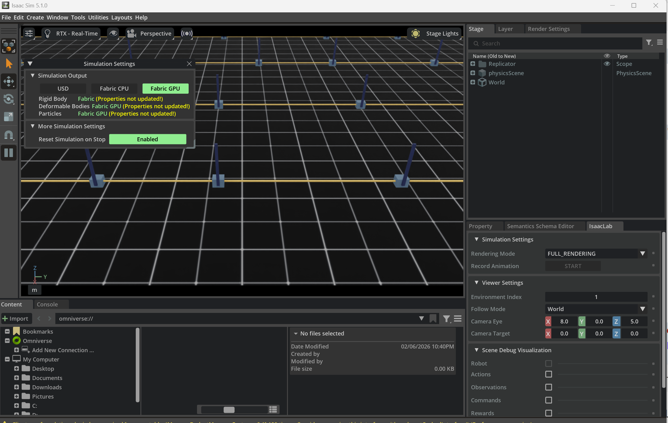
Figure: once world generation enters the batched-training regime, the main concern is no longer only “what exists in the scene,” but also “how environments are replicated, how physics settings are kept consistent, and how batched worlds remain inspectable and debuggable.”
11. Sim2Real-Oriented Rule Design
11.1 Why world rules must serve transfer
A world is not valuable merely because it is internally consistent. It is valuable because it helps policies survive contact with reality.
That means world rules should be judged by whether they improve:
- policy robustness
- calibration tolerance
- latency tolerance
- cross-device generalization
- behavior consistency after deployment
11.2 Physics randomization
Typical physics randomization dimensions:
| Parameter | Examples |
|---|---|
| friction | table, fingertip, object surfaces |
| restitution | floor, object collisions |
| mass | payload or object identity variation |
| center of mass | partially filled or asymmetric objects |
| motor strength | actuator performance variation |
11.3 Visual randomization
Visual randomization usually covers:
- textures
- albedo
- roughness
- lighting intensity
- lighting direction
- camera pose perturbation
- background clutter
The goal is not to maximize chaos. It is to capture plausible real-world variation.
11.4 Sensor randomization
| Sensor dimension | Example |
|---|---|
| camera intrinsics | focal length or principal point perturbation |
| camera extrinsics | mounting error |
| latency | variable frame arrival delay |
| depth noise | range-dependent disturbance |
| IMU bias | bias and drift |
11.5 Delay modeling
Control and sensing delays are often ignored until deployment, where they immediately become visible.
A simple control-delay model is:
where the policy acts on delayed observations. This alone can change manipulation stability or locomotion balance.
11.6 System identification and default parameters
Randomization is not a substitute for identification. Start from the best system-identified default values you can get, then randomize around them.
11.7 The reality-gap loop
graph LR
    A[Real robot traces] --> B[Gap diagnosis]
    B --> C[World parameter update]
    C --> D[Retraining / reevaluation]
    D --> E[Real deployment]
    E --> A
The transfer loop is iterative, not one-shot.
11.8 Sim2Real checklist
| Check | Why it matters |
|---|---|
| randomization ranges justified | prevents unphysical training worlds |
| delays modeled | closes one of the most common sim-real gaps |
| identification baseline exists | keeps randomization centered on reality |
| failure traces fed back | makes the loop evidence-driven |
For broader transfer strategy, see Sim2Real.
12. Platform Implementation Differences
12.1 Why the same world behaves differently across engines
Even when geometry and task logic are nominally identical, engines differ in:
- contact generation
- constraint solving
- actuation abstractions
- time stepping
- sensor pipelines
- scene graph semantics
So "same world" rarely means "same behavior."
12.2 PhysX vs MuJoCo vs DART/Bullet/ODE vs SAPIEN/PhysX
| Engine family | Typical character |
|---|---|
| PhysX | production-oriented, broad feature set, strong Isaac ecosystem |
| MuJoCo | research-friendly, rich contact tuning, compact models |
| Bullet / ODE / DART | broad historical ecosystem, varied strengths by project |
| SAPIEN / PhysX | manipulation-centric workflows with PhysX backend |
12.3 Difference block 1: contact
| Question | Engine-specific consequence |
|---|---|
| when does contact begin? | affected by contact margins and solver thresholds |
| how many contact points exist? | changes grasp stability and stacking |
| how rigid is the solve? | changes jitter and penetration tolerance |
12.4 Difference block 2: joints and drives
| Question | Engine-specific consequence |
|---|---|
| is drive position-based or torque-based under the hood? | changes controller meaning |
| how are limits softened? | changes behavior near boundaries |
| how are mimic or tendon constraints implemented? | changes articulation realism |
12.5 Difference block 3: sensors
| Question | Engine-specific consequence |
|---|---|
| is rendering physically grounded enough? | changes visual transfer |
| how is depth produced? | changes holes and edge behavior |
| what timing model is used? | changes synchronization behavior |
12.6 Difference block 4: world organization
| Question | Engine-specific consequence |
|---|---|
| scene graph or worldbody? | changes modularity and referencing |
| plugin model or script hooks? | changes maintainability |
| can layers / references be used? | changes asset reuse strategy |
12.7 What platform differences imply in practice
Platform migration often requires:
- retuning contact and actuation
- rewriting world loading logic
- changing sensor assumptions
- regenerating benchmark baselines
Do not assume that moving assets is enough.
13. World Validation and Benchmarks
13.1 What to validate
World validation has at least four layers:
- physical plausibility
- task correctness
- numerical stability
- training usefulness
13.2 Validation hierarchy
graph TD
    A[Asset sanity] --> B[Single-scene world validation]
    B --> C[Task validation]
    C --> D[Batch randomization validation]
    D --> E[Training validation]
    E --> F[Transfer validation]
13.3 Core metrics
| Metric | Why it matters |
|---|---|
| success rate | confirms task semantics |
| reset success rate | exposes brittle initialization |
| contact stability | exposes physics tuning issues |
| reproducibility under seed | exposes nondeterminism |
| throughput | matters for training cost |
| trajectory replay consistency | matters for debugging and evaluation |
13.4 Replay and visualization
Replay is essential because many failures are transient:
- one-frame penetrations
- delayed sensor-control mismatch
- reset-only explosions
- rare clutter arrangements
13.5 Why benchmarks matter
Benchmarks force three kinds of discipline:
- task definitions become explicit
- success metrics become comparable
- world assumptions become inspectable
13.6 Validation checklist
| Check | Target |
|---|---|
| seed replay | same seed, same rollout class |
| gravity settling | stable rest state |
| scripted baseline | non-learning controller can execute the obvious path |
| batched reset | no rare environment explosions |
| sensor export | timestamps and calibration consistent |
14. Typical World Templates
14.1 Tabletop grasping world
| Item | Typical choice |
|---|---|
| assets | arm, gripper, tabletop, graspable objects, distractors |
| rule focus | stable resting contact, grasp friction, camera placement |
| common failure | object jitter or grasp succeeds only visually |
14.2 Drawer manipulation world
| Item | Typical choice |
|---|---|
| assets | arm, drawer cabinet, handle, tabletop or housing |
| rule focus | prismatic joints, handle contact, partial occlusion |
| common failure | drawer joints or collisions fight each other |
14.3 Peg insertion / assembly world
| Item | Typical choice |
|---|---|
| assets | peg, hole, fixtures, force sensing, wrist camera |
| rule focus | tight tolerances, contact margins, alignment |
| common failure | tunneling or solver jitter at insertion |
14.4 Quadruped terrain world
| Item | Typical choice |
|---|---|
| assets | quadruped robot, procedural terrain, inertial body |
| rule focus | foot-ground contact, latency, actuator limits |
| common failure | unstable gait due to contact or time mismatch |
14.5 Humanoid carrying world
| Item | Typical choice |
|---|---|
| assets | humanoid, payload, support surface, balance controller |
| rule focus | whole-body inertia, contact sequencing, payload shifts |
| common failure | physically implausible balance because payload modeling is wrong |
14.6 Mobile navigation world
| Item | Typical choice |
|---|---|
| assets | mobile base, static map, dynamic obstacles, range sensors |
| rule focus | localization frames, sensor timing, collision margins |
| common failure | planner works in sim but timing and sensing drift in deployment |
14.7 Reusing templates
Good templates are reusable because they separate:
- asset pools
- world layout logic
- task logic
- validation scripts
15. Development Flow and Checklists
15.1 Engineering flow from empty world to benchmark
flowchart TD
    A[Define task] --> B[Choose asset sources]
    B --> C[Build minimal world]
    C --> D[Validate frames and contact]
    D --> E[Add sensors and task logic]
    E --> F[Add reset and randomization]
    F --> G[Run smoke tests]
    G --> H[Scale to batched training]
    H --> I[Benchmark and transfer]
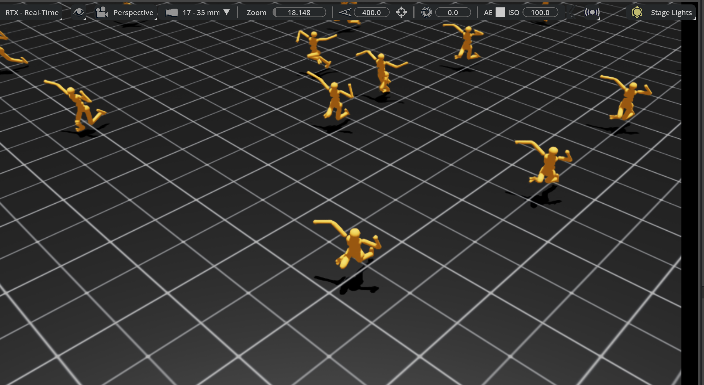
Figure: in real training systems, a “world” is often not a single scene but a batch of replicated episode containers. What matters operationally is whether those worlds can reset, roll out, and emit metrics reliably at scale.
15.2 Recommended development cadence
- build the smallest world that can express the task
- make it stable without learning
- add only one major source of randomness at a time
- benchmark scripted and learned baselines separately
- only then scale environment count or visual fidelity
15.3 What CI / smoke tests should include
| Test | Purpose |
|---|---|
| world load test | catches broken asset refs |
| gravity settle test | catches unstable mass / collision configs |
| reset loop test | catches episodic corruption |
| sensor export test | catches timing or frame mismatch |
| short batched rollout | catches parallel-only failures |
15.4 Failure case 1: bad world config leads training to learn the wrong thing
Typical pattern:
- object collision proxy is larger than visual mesh
- the policy learns to "hover-grasp"
- evaluation in the real world fails because the true object is never actually contacted
Root cause:
- training reward aligned to the wrong world geometry
Fix:
- audit collision vs visual meshes
- log contact points explicitly
- validate scripted grasps against the real object
15.5 Failure case 2: wrong timing model causes deployment jitter
Typical pattern:
- policy is stable in simulation
- deployment shows oscillation or delayed correction
- root cause turns out to be observation latency not modeled in the world
Fix:
- measure end-to-end sensing and actuation latency on hardware
- inject matching delay in simulation
- revalidate controller frequency assumptions
15.6 Final checklist
| Area | Final question |
|---|---|
| assets | are geometry, collision, and semantics consistent? |
| frames | are all transforms explicit and testable? |
| physics | do objects settle, contact, and move plausibly? |
| timing | are control, render, and sensor rates explicit? |
| reset | can the world recover cleanly for thousands of episodes? |
| randomization | are ranges plausible instead of arbitrary? |
| validation | do replay and scripted baselines exist? |
16. Relationship to Other Notes
- For simulator selection and platform positioning, see Simulation Platforms.
- For how robot, object, sensor, and scene assets are modeled and imported, see Simulation Assets.
- For URDF, MJCF, SDF, USD, and surrounding tooling, see Development Toolchain.
- For transfer strategy and domain randomization principles, see Sim2Real.
- For the robot-side control abstractions that world rules ultimately serve, see Control Theory.
17. References and Further Reading
- NVIDIA Isaac Sim and Isaac Lab documentation
- MuJoCo documentation
- Open Robotics SDFormat documentation
- OpenUSD documentation
- ManiSkill, SAPIEN, and robosuite papers and docs
- benchmark papers such as RLBench, LIBERO, and SIMPLER
- Simulation Platforms
- Simulation Assets
- Development Toolchain