CNN Architectures
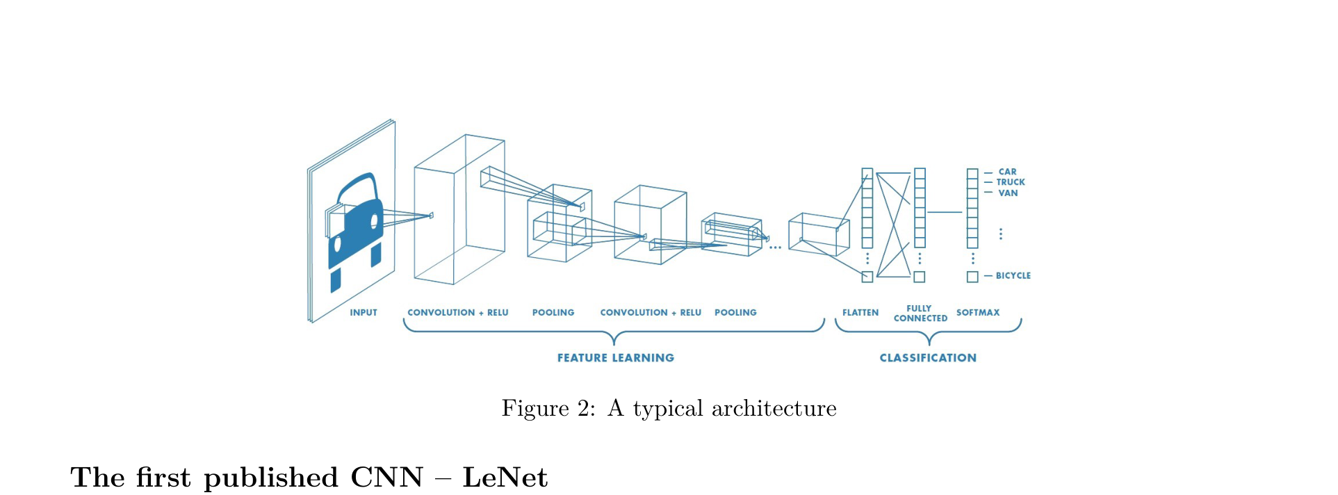
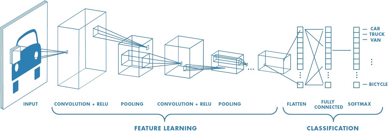
Typical CNN Architecture Pattern
A typical CNN consists of two parts: convolutional blocks (Feature Learning) and a classification head (Classification). Each convolutional block follows this pattern:
[Conv] -> [Activation] -> [Conv] -> [Activation] -> [Pooling]
The model parameters include the weights of all convolutional filters and the parameters of the fully connected layers.
How to Read Network Architecture Diagrams
When reading or designing CNN architectures, pay attention to the following notation conventions:
- The input shape is determined by the preceding layer
- Dense layer:
[Dense, output-size]— a fully connected layer with a specified output size - Convolutional layer:
[Conv, output-channel, padding-size, stride]— a convolutional layer with specified output channels, padding, and stride
LeNet-5
LeCun et al., "Gradient-Based Learning Applied to Document Recognition", 1998
LeNet-5 is the pioneer of CNNs. Proposed by Yann LeCun in 1998 for handwritten digit recognition (MNIST), it established the fundamental paradigm of Convolution (Conv) → Pooling → Fully Connected (FC).
Architecture:
[Input 28×28] -> [Conv 5×5, 6 filters] -> [Activation] -> [Pool 2×2]
             -> [Conv 5×5, 16 filters] -> [Activation] -> [Pool 2×2]
             -> [FC 120] -> [FC 84] -> [Output 10]
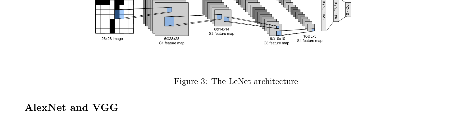
Key Contributions:
- First demonstration of the effectiveness of convolution + pooling
- Established the two-stage paradigm of "feature extraction → classification"
- Due to limited computational resources at the time, LeNet could not be scaled to larger image tasks
AlexNet
Krizhevsky et al., "ImageNet Classification with Deep Convolutional Neural Networks", NeurIPS 2012
In 2012, AlexNet won the ImageNet competition by a dominant margin (reducing the top-5 error rate from 25.8% to 16.4%), marking the beginning of deep learning's dominance in computer vision. AlexNet was the first modern CNN, with each layer designed individually — the concept of "blocks" had not yet emerged.
Architecture (bottom to top):
[Input 224×224×3]
  -> [Conv 11×11, 96, stride 4] -> [ReLU] -> [MaxPool 3×3, stride 2]
  -> [Conv 5×5, 256, pad 2]     -> [ReLU] -> [MaxPool 3×3, stride 2]
  -> [Conv 3×3, 384, pad 1]     -> [ReLU]
  -> [Conv 3×3, 384, pad 1]     -> [ReLU]
  -> [Conv 3×3, 256, pad 1]     -> [ReLU] -> [MaxPool 3×3, stride 2]
  -> [FC 4096] -> [Dropout] -> [FC 4096] -> [Dropout] -> [FC 1000]
Key Contributions:
- ReLU activation function: First large-scale use of ReLU in place of Sigmoid/Tanh in CNNs, addressing the vanishing gradient problem and achieving approximately 6x faster training
- Dropout: Applied Dropout (p=0.5) in the fully connected layers to prevent overfitting
- GPU training: First use of GPUs (2x GTX 580) for distributed training
- Data augmentation: Employed random cropping, horizontal flipping, color jittering, and other augmentation techniques
- LRN (Local Response Normalization): Simulated lateral inhibition in biological neurons (later superseded by BatchNorm)
Limitations: The first layer used an oversized 11×11 convolution kernel with stride 4, causing significant spatial information loss; the fully connected layers accounted for over 95% of the total parameters.
VGGNet
Simonyan & Zisserman, "Very Deep Convolutional Networks for Large-Scale Image Recognition", ICLR 2015
VGGNet (2014) demonstrated the importance of depth — given the same computational resources, increasing depth is more effective than increasing width.
Core Idea — Block Structure:
VGG introduced the concept of block structure, elevating network design to a higher level of abstraction. Each VGG block consists of several \(3 \times 3\) convolutions (padding=1) followed by a \(2 \times 2\) MaxPooling layer (stride=2):
VGG Block:
  [3×3 Conv, pad 1] -> [ReLU]
  [3×3 Conv, pad 1] -> [ReLU]
  [2×2 MaxPool, stride 2]
Why use 3×3 instead of larger kernels?
- Two stacked \(3 \times 3\) convolutions have the same receptive field as a single \(5 \times 5\) convolution
- Three stacked \(3 \times 3\) convolutions are equivalent to a single \(7 \times 7\)
- But with fewer parameters: \(3 \times (3^2 C^2) = 27C^2\) < \(7^2 C^2 = 49C^2\)
- Meanwhile, more nonlinearities are introduced (more ReLU layers), yielding stronger representational power
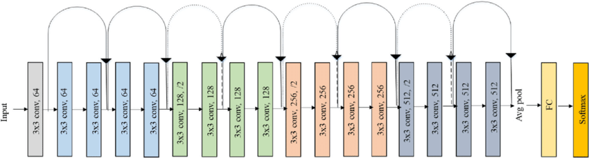
VGG-16 Architecture:
| Stage | Layers | Channels | Output Size |
|---|---|---|---|
| Block 1 | 2×Conv | 64 | 112×112 |
| Block 2 | 2×Conv | 128 | 56×56 |
| Block 3 | 3×Conv | 256 | 28×28 |
| Block 4 | 3×Conv | 512 | 14×14 |
| Block 5 | 3×Conv | 512 | 7×7 |
| Head | 3×FC | 4096, 4096, 1000 | — |
Limitations: Extremely large parameter count (VGG-16 has approximately 138 million parameters), with the fully connected layers accounting for over 80%. Training and inference are relatively slow.
Inception / GoogLeNet
Szegedy et al., "Going Deeper with Convolutions", CVPR 2015
GoogLeNet (2014) did not merely deepen the network — it widened it. The core idea is to use convolution kernels of different sizes simultaneously within the same layer, allowing the network to learn which scale is most effective on its own.
Inception Module:
         Input
       /   |   \    \
   1×1   3×3   5×5  MaxPool
   Conv  Conv  Conv  3×3
       \   |   /    /
        Concatenate
          Output
A \(1 \times 1\) convolution is applied before each branch for channel dimensionality reduction, drastically lowering the computational cost:
         Input (256ch)
       /       |        \        \
   1×1(64)  1×1(96)   1×1(16)  MaxPool
              |          |        |
           3×3(128)   5×5(32)  1×1(32)
       \       |        /        /
            Concatenate (256ch)
Key Contributions:
- Multi-scale feature extraction: Parallel use of \(1 \times 1\), \(3 \times 3\), and \(5 \times 5\) convolutions within the same layer
- The power of \(1 \times 1\) convolutions: Used as bottleneck layers for channel dimensionality reduction, cutting computational cost by an order of magnitude
- Global Average Pooling: Replaced large fully connected layers with global average pooling; GoogLeNet has only about 5 million parameters (1/27 of VGG)
- Auxiliary classifiers: Added auxiliary losses at intermediate layers to alleviate vanishing gradients in deep networks
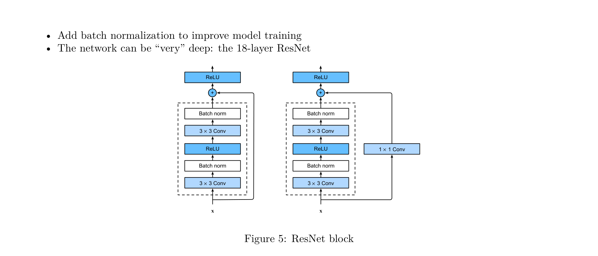
ResNet
He et al., "Deep Residual Learning for Image Recognition", CVPR 2016
When networks exceed 20 layers, the vanishing gradient and degradation problems cause performance to actually decline — this is not overfitting, as even the training error is higher for deeper networks. In 2015, Kaiming He proposed ResNet, introducing residual connections (skip connections) that made it possible to train networks with hundreds or even thousands of layers.
ResNet is the core backbone of modern CNNs. Most subsequent architectures are essentially improvements built upon it. Its significance is on par with backpropagation and the Attention mechanism.
Core Formula:
That is: the output of a layer = the layer's computation + the original input.
Why do residual connections work?
- Direct gradient flow: During backpropagation, gradients can flow directly back to earlier layers through the skip connections, alleviating vanishing gradients
- Identity mapping as a fallback: If a layer does not need to learn any additional transformation, \(F(x)\) can learn to be zero, making the output simply \(x\) (an identity mapping). This is much easier than having the network learn an identity function from scratch
- Ensemble perspective: ResNet can be viewed as an ensemble of many paths of different depths
ResNet residual blocks come in two forms:
- Basic Block:
x -> [3×3 Conv] -> [BN] -> [ReLU] -> [3×3 Conv] -> [BN] -> (+x) -> [ReLU] - Bottleneck Block (with 1×1 projection): When the input and output dimensions differ, a
1×1 Convis used to project \(x\) to the matching dimension before addition
ResNet-18 Architecture:
| Stage | Residual Blocks | Channels | Output Size |
|---|---|---|---|
| Conv1 | 1×Conv 7×7, stride 2 | 64 | 112×112 |
| Pool | MaxPool 3×3, stride 2 | 64 | 56×56 |
| Stage 1 | 2×BasicBlock | 64 | 56×56 |
| Stage 2 | 2×BasicBlock | 128 | 28×28 |
| Stage 3 | 2×BasicBlock | 256 | 14×14 |
| Stage 4 | 2×BasicBlock | 512 | 7×7 |
| Head | AvgPool + FC | 1000 | — |
A key design choice in ResNet is the inclusion of Batch Normalization after every convolutional layer to improve training.
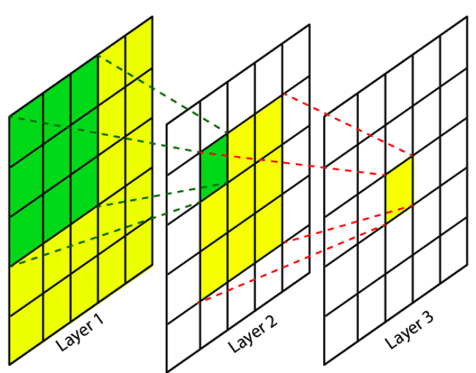
Receptive Field: The region in the input image that corresponds to a particular output unit. By stacking multiple layers of small convolution kernels, the receptive field grows progressively larger.
DenseNet
Huang et al., "Densely Connected Convolutional Networks", CVPR 2017
While ResNet solved the problem of "training deeper networks," DenseNet went further by addressing "no feature goes to waste."
Core Idea — Dense Connection:
In DenseNet, every layer receives feature maps from all preceding layers as input, not just the immediately previous one:
x0 → x1 → x2 → x3 → x4
 └────┘    |    |    |
 └─────────┘    |    |
 └──────────────┘    |
 └───────────────────┘
That is, the input to layer \(\ell\) is the concatenation of all preceding layers' outputs: \(x_\ell = H_\ell([x_0, x_1, \ldots, x_{\ell-1}])\)
Dense Block:
Dense Block:
  Layer 1: BN -> ReLU -> 1×1 Conv(4k) -> BN -> ReLU -> 3×3 Conv(k)
  Layer 2: receives [x0, x1] as input
  Layer 3: receives [x0, x1, x2] as input
  ...
Here \(k\) is called the growth rate, meaning each layer adds only \(k\) new channels. Between Dense Blocks, a Transition Layer (\(1 \times 1\) Conv + \(2 \times 2\) AvgPool) is used for downsampling and channel compression.
Key Contributions:
- Feature reuse: All feature maps are shared with all subsequent layers, preventing information loss
- Parameter efficiency: Thanks to feature reuse, each layer only needs to learn a small number of new features (\(k\) is typically 12 or 32), resulting in far fewer parameters than ResNet
- Implicit deep supervision: Shallow features can be directly accessed by deeper layers and the loss function, producing an effect similar to auxiliary losses
- Smooth gradient flow: Every layer has a "short path" to the loss, making training more stable
MobileNet Series
Howard et al., "MobileNets: Efficient Convolutional Neural Networks for Mobile Vision Applications", 2017
MobileNet is designed specifically for mobile and embedded devices. Its core innovation is the Depthwise Separable Convolution.
Standard Convolution vs. Depthwise Separable Convolution:
Computational cost of standard convolution: \(k^2 \times C_{in} \times C_{out} \times H \times W\)
Depthwise separable convolution decomposes it into two steps:
Standard Convolution (single-step):
  Input [H×W×Cin] --[k×k×Cin×Cout]--> Output [H×W×Cout]

Depthwise Separable Convolution (two steps):
  Step 1 - Depthwise Conv (independent convolution per channel):
    Input [H×W×Cin] --[k×k×1×Cin]--> [H×W×Cin]
  Step 2 - Pointwise Conv (1×1 convolution to mix channels):
    [H×W×Cin] --[1×1×Cin×Cout]--> Output [H×W×Cout]
Computational Cost Comparison:
For \(3 \times 3\) convolutions, the computational cost is approximately \(\frac{1}{8} \sim \frac{1}{9}\) that of standard convolutions.
MobileNet V2 Improvements:
Introduced the Inverted Residual Block:
Inverted Residual Block:
  Input(thin) -> [1×1 Conv expand] -> [BN+ReLU6]
              -> [3×3 Depthwise Conv] -> [BN+ReLU6]
              -> [1×1 Conv compress] -> [BN]
              -> (+Input)
This is the opposite of ResNet's residual block: MobileNet V2 "expands" in the middle (thin → fat → thin), while ResNet "compresses" in the middle (fat → thin → fat).
ShuffleNet
Zhang et al., "ShuffleNet: An Extremely Efficient Convolutional Neural Network for Mobile Devices", CVPR 2018
ShuffleNet further optimizes upon MobileNet by introducing the Channel Shuffle operation.
Problem: Although Group Convolution reduces computational cost, each group operates in isolation with no cross-group information exchange, limiting feature expressiveness.
Solution — Channel Shuffle:
Channel shuffle after group convolution:
  Group 1: [a1, a2, a3]     After shuffle:  [a1, b1, c1]
  Group 2: [b1, b2, b3]  ------------>      [a2, b2, c2]
  Group 3: [c1, c2, c3]                     [a3, b3, c3]
By rearranging the channel order, information from different groups can mix and interact in the next layer, with virtually no additional computational cost.
Key Contributions:
- Channel Shuffle: Enables cross-group information exchange with zero computational overhead
- Pointwise Group Convolution: Applies grouping to \(1 \times 1\) convolutions as well, further reducing computational cost
- Achieves higher accuracy than MobileNet V1 under the same computational budget
Summary of CNN Architecture Evolution
| Year | Architecture | Depth | Core Innovation | ImageNet Top-5 |
|---|---|---|---|---|
| 1998 | LeNet-5 | 5 | Conv+Pool paradigm | — |
| 2012 | AlexNet | 8 | ReLU, Dropout, GPU | 16.4% |
| 2014 | VGGNet | 16/19 | Stacked 3×3 small kernels, block structure | 7.3% |
| 2014 | GoogLeNet | 22 | Inception module, 1×1 convolution | 6.7% |
| 2015 | ResNet | 152+ | Residual connections | 3.6% |
| 2017 | DenseNet | 121+ | Dense connections, feature reuse | — |
| 2017 | MobileNet | 28 | Depthwise separable convolution | — |
| 2018 | ShuffleNet | — | Channel shuffle | — |
Evolution Trajectory:
- Going deeper: LeNet(5) → AlexNet(8) → VGG(19) → ResNet(152+)
- Getting smarter: Inception (multi-scale) → ResNet (residual) → DenseNet (dense connections)
- Getting lighter: MobileNet (depthwise separable) → ShuffleNet (channel shuffle)