Optimizer

First, note that "optimization" and "optimizer" are two distinct concepts.

Optimizers are broadly divided into first-order and second-order optimizers.

First-Order Optimizers have evolved chronologically as follows:

1. Vanilla Gradient Descent: Gradient Descent (1847), SGD (1951)
2. With Momentum: Polyak Momentum (1964), Nesterov Momentum (1983)
3. With Adaptive Learning Rate: AdaGrad (2011), RMSProp (2012), AdaDelta (2012)
4. Combining Momentum and Adaptive Gradient: Adam (2014), AdamW (2017)

Second-Order Optimizers have evolved chronologically as follows:

1. Pure Second-Order: Newton's Method (17th century), Quasi-Newton L-BFGS (1989)
2. Approximate Second-Order: KFAC (2015), AdaHessian (2020)

SGD

We have already covered gradient descent in detail in the optimization theory notes. Since SGD serves as the foundation for all subsequent optimizers, we briefly review the key ideas here.

Gradient Descent in One Dimension

One-dimensional gradient descent provides valuable intuition. Consider a class of continuously differentiable real-valued functions \(f : \mathbb{R} \to \mathbb{R}\). Using the Taylor expansion, we obtain

\[ f(x+\epsilon)=f(x)+\epsilon f'(x)+O(\epsilon^2) \]

That is, to first-order approximation, \(f(x+\epsilon)\) can be expressed in terms of the function value \(f(x)\) and the first derivative \(f'(x)\) at \(x\).

We can assume that moving a small amount \(\epsilon\) in the direction of the negative gradient will decrease \(f\). For simplicity, we choose a fixed step size \(\eta>0\) and set

\[ \epsilon=-\eta f'(x) \]

Substituting into the Taylor expansion, we get

\[ f(x-\eta f'(x)) = f(x)-\eta f'^2(x)+O(\eta^2 f'^2(x)) \]

If the derivative \(f'(x)\neq 0\) does not vanish, we can proceed with the expansion, because

\[ \eta f'^2(x)>0 \]

Moreover, we can always choose \(\eta\) small enough so that the higher-order terms become negligible. Therefore,

\[ f(x-\eta f'(x)) \lesssim f(x) \]

This means that if we iterate \(x\) using the update rule

\[ x \leftarrow x-\eta f'(x) \]

the value of \(f(x)\) can decrease.

Thus, in gradient descent, we first choose an initial value \(x\) and a constant \(\eta>0\), then iteratively update \(x\) until a stopping condition is met — for example, when the magnitude of the gradient \(|f'(x)|\) becomes sufficiently small or when the number of iterations reaches a prescribed limit.

Let us illustrate gradient descent with a concrete example. For simplicity, we choose the objective function

\[ f(x)=x^2. \]

Although we know that \(f(x)\) attains its minimum at \(x=0\), we still use this simple function to observe how \(x\) evolves.

Stochastic Gradient Update

In deep learning, the objective function is typically the average of the loss functions over all training samples. Given a training dataset of \(n\) samples, let \(f_i(\mathbf{x})\) denote the loss function for the \(i\)-th training sample, where \(\mathbf{x}\) is the parameter vector. The objective function is then

\[ f(\mathbf{x}) = \frac{1}{n} \sum_{i=1}^{n} f_i(\mathbf{x}). \]

The gradient of the objective function with respect to \(\mathbf{x}\) is

\[ \nabla f(\mathbf{x}) = \frac{1}{n} \sum_{i=1}^{n} \nabla f_i(\mathbf{x}). \]

If we use full gradient descent, the computational cost per iteration is \(O(n)\), which grows linearly with \(n\). When the training dataset is large, this makes each iteration of gradient descent expensive.

Stochastic gradient descent (SGD) reduces the per-iteration computational cost. At each iteration of SGD, we uniformly sample a random index \(i\), where \(i \in \{1, \dots, n\}\), and compute the gradient \(\nabla f_i(\mathbf{x})\) to update \(\mathbf{x}\):

\[ \mathbf{x} \leftarrow \mathbf{x} - \eta \nabla f_i(\mathbf{x}), \]

where \(\eta\) is the learning rate. The per-iteration cost drops from \(O(n)\) for gradient descent to \(O(1)\).

Furthermore, we emphasize that the stochastic gradient \(\nabla f_i(\mathbf{x})\) is an unbiased estimate of the full gradient \(\nabla f(\mathbf{x})\), since

\[ \mathbb{E}_i \nabla f_i(\mathbf{x}) = \frac{1}{n} \sum_{i=1}^{n} \nabla f_i(\mathbf{x}) = \nabla f(\mathbf{x}). \]

This means that, on average, the stochastic gradient is a good estimate of the full gradient.

Convergence Conditions for SGD

The convergence of SGD is highly sensitive to the choice of learning rate. According to the Robbins–Monro conditions, SGD convergence requires the learning rate \(\epsilon_k\) to satisfy the following two conditions:

\[ \sum_{k=1}^{\infty} \epsilon_k = \infty \quad \text{and} \quad \sum_{k=1}^{\infty} \epsilon_k^2 < \infty \]

The first condition ensures that the sum of learning rates diverges, guaranteeing that the algorithm has enough "energy" to reach an arbitrarily distant optimum. The second condition ensures that the sum of squared learning rates converges, keeping the cumulative effect of noise bounded so that the algorithm can ultimately converge.

Note: A constant learning rate \(\epsilon_k = \epsilon\) violates the second condition (\(\sum \epsilon^2 = \infty\)), so theoretically, SGD with a constant learning rate is not guaranteed to converge. This is why learning rate decay schedules are commonly used in practice. A typical approach is to halve the learning rate or reduce it by a factor of \(\frac{1}{10}\) when training loss plateaus.

Problems with SGD

The gradient direction in SGD does not always point toward the optimum. Recall the quadratic "bowl" example: the gradient direction typically does not point directly toward the minimum \((0,0)\) but deviates from it. The degree of deviation depends on the problem structure — specifically, on the condition number of the Hessian matrix. A larger condition number leads to greater deviation between the gradient direction and the optimal direction, resulting in slower convergence.

Dynamic Learning Rate

Replacing the constant \(\eta\) with a time-dependent learning rate \(\eta(t)\) adds complexity to controlling the convergence of the optimization algorithm. In particular, we need to determine the appropriate decay rate for \(\eta\). If it decays too quickly, we stop optimizing prematurely. If it decays too slowly, we waste time on optimization. The following are some basic strategies for adjusting \(\eta\) over time (more advanced strategies will be discussed later):

\[ \eta(t) = \eta_i \quad \text{if } t_i \le t \le t_{i+1} \qquad \text{Piecewise constant} \]

\[ \eta(t) = \eta_0 \cdot e^{-\lambda t} \qquad \text{Exponential decay} \]

\[ \eta(t) = \eta_0 \cdot (\beta t + 1)^{-\alpha} \qquad \text{Polynomial decay} \]

In the first piecewise constant scenario, we reduce the learning rate — for example, whenever optimization progress stalls. This is a common strategy for training deep networks. Alternatively, exponential decay reduces the rate more aggressively. Unfortunately, this often leads to premature stopping before the algorithm converges.

A popular choice is polynomial decay with \(\alpha = 0.5\). For convex optimization, there is substantial evidence that this decay rate performs well.

Sampling Without Replacement

In theory, stochastic gradient descent assumes that we draw samples from a continuous distribution \(p(x,y)\). For a finite dataset, we should theoretically sample from \(n\) samples "with replacement." However, in engineering practice, we typically shuffle the \(n\) samples and iterate through them sequentially. This is called sampling without replacement.

More specifically, we typically perform a global shuffle followed by batching for training — we refer to this process as "batching."

The standard industrial pipeline for batching typically consists of four steps:

1. Shuffle: At the beginning of each epoch, randomly permute all data indices.
2. Partition: Divide the index sequence into contiguous segments of size \(B\) (the batch_size).
3. Collate: Stack the \(B\) samples (e.g., images, text) into a single tensor. For example, \(B\) images of shape \((3, 224, 224)\) are packed into a \((B, 3, 224, 224)\) matrix.
4. Update: Compute the average gradient over the batch and update the model parameters.

If Batch Size = total dataset size \(n\), this reduces to full gradient descent; if Batch Size = 1, it becomes the purely theoretical SGD. In practice, we typically choose Batch Size = 32, 64, 128, etc. This approach is also known as mini-batch SGD (MB-SGD).

---

Below we briefly argue why sampling without replacement is viable in practice.

Suppose we sample \(x_i\) (typically with labels \(y_i\)) from a distribution \(p(x,y)\) and use it to update the model parameters in some fashion.

In particular, for a finite number of samples, we only discuss a discrete distribution composed of functions \(\delta_{x_i}\) and \(\delta_{y_i}\) that allow us to perform stochastic gradient descent on:

\[ p(x,y) = \frac{1}{n} \sum_{i=1}^{n} \delta_{x_i}(x)\delta_{y_i}(y). \]

However, this is not exactly what we do in practice. In the simple examples in this section, we merely add noise to otherwise non-random gradients — that is, we pretend we have pairs \((x_i, y_i)\). It turns out this is justified here (see the exercises for a detailed discussion).

A more subtle issue is that, in all previous discussions, we did not actually sample with replacement. Instead, we traversed all instances exactly once. To understand why this is preferable, consider the reverse: sampling \(n\) observations with replacement from a discrete distribution. The probability of randomly selecting element \(i\) is \(1/n\). Therefore, the probability of selecting it at least once is

\[ P(\text{choose } i) = 1 - P(\text{omit } i) = 1 - \left(1 - \frac{1}{n}\right)^n \approx 1 - e^{-1} \approx 0.63. \]

A similar argument shows that the probability of picking a given sample exactly once is

\[ \binom{n}{1} \frac{1}{n} \left(1 - \frac{1}{n}\right)^{n-1} = \frac{n}{n-1} \left(1 - \frac{1}{n}\right)^n \approx e^{-1} \approx 0.37. \]

This leads to increased variance and reduced data efficiency compared to sampling without replacement. Therefore, in practice we use the latter (which is the default choice in the D2L textbook). One final note: when repeatedly cycling through the training dataset, we traverse it in a different random order each time.

Batch Size

As mentioned above, in practice we use mini-batch gradient descent rather than pure theoretical SGD. Generally, we choose the largest Batch Size that hardware constraints allow. The primary hardware bottleneck for Batch Size is GPU memory. We prefer powers of 2 (32, 64, 128, ...) because GPU hardware alignment optimizations (CUDA Cores) are most efficient at these values.

An important rule of thumb: when you scale batch_size by a factor of \(k\), you should also scale the learning rate by the same factor \(k\). This is because larger batches produce more accurate gradient estimates (less noise), allowing for larger step sizes.

In practice, 128 is often a good starting point for most CNN and NLP tasks. Then we can observe the loss curve:

• If the loss oscillates wildly and fails to converge, try increasing the batch size or reducing the learning rate.
• If the loss decreases too slowly, try increasing the learning rate.

Additionally, we can use gradient accumulation: for instance, if the hardware cannot support a batch size of 32, we can run 4 forward-backward passes with batch=8, accumulate the gradients over 4 steps, and then perform a single update — logically equivalent to batch=32.

Momentum

The k-step Method: A Unifying Framework

Before introducing momentum methods, we first establish a unifying theoretical framework: k-step methods (Polyak, 1962).

Our goal is to solve the equation \(\nabla J(\theta) = 0\). This typically requires an iterative numerical algorithm that produces a sequence of points:

\[ \theta^{(0)}, \theta^{(1)}, \theta^{(2)}, \dots, \theta^{(k)}, \dots \]

converging to the optimal solution \(\theta^*\). In such algorithms, each new \(\theta^{(t+1)}\) is computed based on previous iterates \(\theta^{(i)}\).

Definition: A k-step method is one in which the update for \(\theta^{(t+1)}\) depends on the previous \(k\) iterates \(\theta^{(t)}, \theta^{(t-1)}, \dots, \theta^{(t-k+1)}\).

All methods discussed so far — GD, SGD, and AdaGrad — are 1-step methods. By considering k-step methods, convergence can be accelerated as \(k\) increases. However, in practice, acceleration methods primarily use \(k=2\). For \(k>2\), the computational complexity increases significantly, hyperparameter selection becomes more difficult, and the improvement in convergence speed is marginal.

Methods with \(k=2\) are known as accelerated gradient descent or momentum methods.

General update formula for k-step methods (Polyak, 1962):

\[ \theta^{t+1} = \sum_{i=0}^{k-1} \beta_i \theta^{t-i} + \sum_{i=0}^{k-1} \alpha_i \nabla J(\theta^{t-i}) \]

where \(\sum_{i=0}^{k-1} \beta_i = 1\) (to ensure stability).

The 2-step method update formula is:

\[ \theta^{t+1} = (1-\beta)\theta^t + \beta \theta^{t-1} - \alpha_1 \nabla J(\theta^t) - \alpha_2 \nabla J(\theta^{t-1}) \]

\[ = \theta^t - \beta(\theta^t - \theta^{t-1}) - \alpha_1 \nabla J(\theta^t) - \alpha_2 \nabla J(\theta^{t-1}) \]

Polyak Momentum

Momentum, sometimes also called the Heavy Ball Method, was first proposed in 1964 by the Soviet mathematician Boris Polyak. Originally, it was not applied to SGD but to standard GD. Polyak introduced a "heavy ball" concept — mathematically, momentum — that accelerates convergence, especially in ravines or ill-conditioned scenarios.

In elongated, ill-conditioned valleys, SGD oscillates back and forth and makes slow progress. Momentum was designed to address exactly this problem. When updating parameters, momentum takes into account not only the current gradient but also the direction and speed of the previous step. The effect is that when oscillating across the walls of a valley, the left-right gradients partially cancel out due to inertia, thereby suppressing oscillation. Meanwhile, along the flat valley floor where the gradient direction is stable, inertia accumulates steadily, accelerating progress.

In one sentence: Polyak momentum = gradient + inertia.

Derivation of Polyak Momentum: Polyak's method was the first to introduce momentum. It is a 2-step method with the following update formula:

\[ \theta^{t+1} = \theta^t - \alpha \nabla J(\theta^t) + \beta(\theta^t - \theta^{t-1}) \]

This resembles the general 2-step method above but uses only a single gradient term. Rewriting it:

\[ \theta^{t+1} - \theta^t = \beta(\theta^t - \theta^{t-1}) - \alpha \nabla J(\theta^t) \]

Defining the momentum term \(m_t = \theta^{t+1} - \theta^t\), we arrive at the standard form of Polyak momentum:

\[ \begin{cases} m_t = \beta \cdot m_{t-1} - \alpha \cdot g_t \\ \theta^{t+1} = \theta^t + m_t \end{cases} \]

where \(g_t = \nabla J(\theta^t)\), \(\beta\) is the momentum coefficient (momentum factor), and \(\alpha\) is the learning rate. Note that 1-step methods (i.e., vanilla GD) have only \(\theta^{t+1} = \theta^t - \alpha g_t\), with no momentum term.

Intuition for momentum: Consider the gradient vector \(g_t = [g_{t1}, g_{t2}, \dots, g_{tn}]^T\):

• If along some dimension \(i\) the gradient values \(g_{ti}\) consistently have the same sign (consistent direction), then \(m_{ti}\) grows steadily from the accumulated same-direction changes, accelerating updates in that direction.
• If along another dimension \(j\) the gradient values \(g_{tj}\) frequently alternate in sign (oscillation), then \(m_{tj}\) remains small due to positive-negative cancellation, dampening oscillation in that direction.

SGD with Polyak Momentum: Complete Algorithm

Given: Learning rate \(\eta\), momentum coefficient \(\mu\), initial points \(\theta_0, \theta_1\)

Repeat the following steps:

1. Sample a mini-batch \(\{x^{(1)}, x^{(2)}, \dots, x^{(m)}\}\)
2. Compute the gradient: \(\hat{g}_t \leftarrow \frac{1}{m} \sum_{i=1}^{m} \nabla \mathcal{L}(f(x^{(i)}; \theta); y^{(i)})\)
3. Update: - \(m_t \leftarrow \mu \cdot m_{t-1} - \eta \cdot \hat{g}_t\) (momentum) - \(\theta_{t+1} \leftarrow \theta_t + m_t\) (parameters)
4. \(t \leftarrow t + 1\)

Until the stopping criterion is met. The learning rate and momentum coefficient are typically set empirically.

Optimal Polyak Parameters and Condition Number Analysis

Recall that the goal of training a deep neural network is \(\min_\theta J(\theta)\), where \(g = \nabla J(\theta)\) is the gradient vector and \(H = \nabla^2 J(\theta)\) is the Hessian matrix.

Let \(m\) and \(M\) be the smallest and largest eigenvalues (or their bounds) of the Hessian matrix \(H\), i.e.:

\[ mI \preceq H \preceq MI \]

Polyak's optimal hyperparameters are:

\[ \alpha = \frac{4}{(\sqrt{M} + \sqrt{m})^2}, \quad \beta = \left(\frac{\sqrt{M} - \sqrt{m}}{\sqrt{M} + \sqrt{m}}\right)^2 \]

The distance to the optimum then satisfies:

\[ \|\theta^t - \theta^*\| \le c \cdot \left(\frac{\sqrt{M} - \sqrt{m}}{\sqrt{M} + \sqrt{m}} + \varepsilon\right)^t \]

Condition number analysis: Define the condition number \(\rho = \frac{M}{m}\), which measures the "ill-conditioning" of the optimization problem. A larger \(\rho\) means that \(J(\theta)\) varies rapidly in some directions and slowly in others (imagine elliptically stretched contour lines). A small \(\rho\) indicates a well-conditioned problem (circular contour lines).

Convergence comparison between SGD and Polyak Momentum:

	SGD (1-step)	Polyak Momentum (2-step)
Update rule	\(\theta^{t+1} = \theta^t - \alpha g_t\)	\(m_t = \beta m_{t-1} - \alpha g_t\), \(\theta^{t+1} = \theta^t + m_t\)
Convergence bound	\(\|\theta^t - \theta^*\| \le c_1 \|\theta^0 - \theta^*\| (q_1 + \varepsilon)^t\)	\(\|\theta^t - \theta^*\| \le c_2 (\|\theta^0 - \theta^*\|^2 + \|\theta^1 - \theta^*\|)^{1/2} (q_2 + \varepsilon)^t\)
Optimal convergence rate	\(q_1 = \frac{M-m}{M+m}\), \(\alpha = \frac{2}{M+m}\)	\(q_2 = \frac{\sqrt{M}-\sqrt{m}}{\sqrt{M}+\sqrt{m}}\)

For a large condition number \(\rho\):

\[ q_2 = \frac{\sqrt{M} - \sqrt{m}}{\sqrt{M} + \sqrt{m}} = \frac{\sqrt{\rho} - 1}{\sqrt{\rho} + 1} \approx 1 - \frac{2}{\sqrt{\rho}} \]

Therefore, to reduce the distance by a factor of \(e^k\), the required number of iterations is:

• SGD: \(t = \frac{k}{\ln q_1} \approx \frac{k\rho}{2}\), i.e., \(O(\kappa)\)
• Polyak Momentum: \(t = \frac{k}{\ln q_2} \approx \frac{k\sqrt{\rho}}{2}\), i.e., \(O(\sqrt{\kappa})\)

Conclusion: Momentum methods improve the convergence rate from \(O(\kappa)\) to \(O(\sqrt{\kappa})\), which represents a dramatic speedup for ill-conditioned problems with large condition numbers.

Nesterov Momentum

Nesterov Momentum (Nesterov's Accelerated Gradient, NAG) was proposed in 1983 by another Soviet mathematician, Yurii Nesterov (later introduced to deep learning by Sutskever in 2013).

This is a clever refinement of Polyak momentum. The core idea is: instead of computing the gradient at the current position, first take a tentative step in the direction of the current momentum to "look ahead," evaluate the gradient at that new position, and then combine it with the momentum to decide the final update.

In one sentence: Nesterov momentum = look-ahead gradient + inertia — smarter than standard momentum.

Mathematical comparison of Polyak (classical) momentum vs. Nesterov momentum:

Polyak momentum computes the gradient at the current position \(\theta_t\):

\[ \begin{cases} m_t = \mu \cdot m_{t-1} - \eta \nabla J(\theta_t) \\ \theta_{t+1} = \theta_t + m_t \end{cases} \]

Nesterov momentum computes the gradient at the look-ahead position \(\theta_t + \mu m_{t-1}\):

\[ \begin{cases} m_t = \mu \cdot m_{t-1} - \eta \nabla J(\theta_t + \mu m_{t-1}) \\ \theta_{t+1} = \theta_t + m_t \end{cases} \]

The key difference lies in where the gradient is evaluated. Polyak computes the gradient at the current point \(\theta_t\), while Nesterov first "looks ahead" one step along the momentum direction to \(\theta_t + \mu m_{t-1}\) and evaluates the gradient there.

Note: In some papers and textbooks, the vector \(m_t\) is denoted \(v_t\) (velocity), but the update rules are identical.

Equivalent form using velocity notation:

Polyak	Nesterov
\(v_t = \mu v_{t-1} - \eta \nabla J(\theta_t)\)	\(v_t = \mu v_{t-1} - \eta \nabla J(\theta_t + \mu v_{t-1})\)
\(\theta_{t+1} = \theta_t + v_t\)	\(\theta_{t+1} = \theta_t + v_t\)

where \(\mu\) is the momentum update factor and \(\eta\) is the learning rate.

Comparison of Polyak and Nesterov

• When the learning rate \(\eta\) is small, the two methods are nearly equivalent in behavior.
• The difference becomes apparent when \(\eta\) is large. Let \(\lambda_1 = \lambda_{\max}(\nabla^2 J)\) be the largest eigenvalue of the Hessian. When \(\eta \cdot \lambda_1 < 1\), Nesterov is more "conservative" than Polyak, taking smaller steps in directions with large gradient variation, and is therefore more stable.
• However, if \(\eta \cdot \lambda_1 > 1\), Nesterov may become overly aggressive and diverge.

Equivalence example (Sutskever, 2013): For the one-dimensional quadratic objective \(J(\theta) = \frac{\lambda}{2}\theta^2 + c\theta\), the gradient is \(g(\theta) = \lambda\theta + c\). The Polyak and Nesterov updates are equivalent in this case if and only if the Nesterov momentum coefficient \(\mu_N\) and the Polyak momentum coefficient \(\mu_P\) satisfy:

\[ \mu_P = \mu_N(1 - \eta\lambda) \]

where \(\lambda\) is the eigenvalue from the objective function \(J(\theta)\).

Nesterov Convergence Guarantee

If \(J(\theta)\) is convex, Nesterov's method (Nesterov, 1983) guarantees:

\[ J(\theta^k) - J(\theta^*) \le \frac{C}{(k+2)^2} \]

where \(C = 4L\|x_{-1} - x^*\|^2\) (\(x_{-1}\) is the initial point). This is the optimal decay rate.

This convergence is achieved by choosing specific momentum coefficients and a learning rate schedule:

\[ \mu_k = \frac{a_k - 1}{a_{k+1}}, \quad a_{k+1} = \frac{1 + \sqrt{4a_k^2 + 1}}{2}, \quad a_0 = 1 \]

\[ \eta_k = \frac{1}{2}\eta_{k-1} \quad \text{(learning rate)} \]

Nesterov proved that after a fixed number of \(N = \lfloor 4\sqrt{M/m} \rfloor - 1\) steps, the objective value is at least halved:

\[ J(\theta_N) - J(\theta^*) \le \frac{1}{2}(J(\theta_{-1}) - J(\theta^*)) \]

This is a linear convergence rate similar to that of Polyak's method (possibly with a different constant slope).

---

Adaptive Gradient

Momentum addresses the problem from the perspective of direction, while adaptive gradient methods address it from the perspective of step size.

AdaGrad

AdaGrad (Adaptive Gradient Algorithm), proposed by Duchi et al. in 2011, was the first optimization algorithm to adaptively adjust the learning rate for each parameter.

Core intuition: During training, different parameters vary greatly in importance and update frequency. For sparse features (e.g., rare words in NLP), the corresponding parameter gradients are rarely nonzero, and when they do appear, they should receive large updates. Conversely, frequently updated parameters should have their step sizes gradually reduced. AdaGrad achieves this by accumulating the sum of squared historical gradients: the more frequently a parameter is updated, the larger the accumulated value, and the smaller the effective learning rate.

High-level idea: AdaGrad is designed to stay close to the GD direction while minimizing a "proximal function," so that the new update direction is more effective at minimizing \(J(\theta)\) than the original GD direction.

Proximal Method Derivation of AdaGrad

Recall the GD update: \(x_{t+1} = x_t + (-\eta g_t)\), where \(v_t = -\eta g_t\) is the GD update vector. AdaGrad seeks a "new" update direction:

\[ x_{t+1} = x_t + u_t \]

where \(u_t\) is the new update vector, required to minimize a proximal function while staying close to \(v_t\):

\[ \min_{u} \quad f(u) + \frac{1}{2t}\|u_t - v_t\|_2^2 \]

Here \(f(u)\) is a chosen convex function, and \(\frac{1}{2t}\) controls how close \(u_t\) stays to \(v_t\).

For AdaGrad, we choose \(f(u_t) = \frac{1}{t}u_t^T H_t u_t\) (where \(H_t\) is a known matrix), and the new update is obtained by solving:

\[ \min_{u_t} \quad \frac{1}{t}u_t^T H_t u_t - 2u_t^T v_t \]

Setting the derivative with respect to \(u_t\) to zero: \(\frac{2}{t}H_t u_t - 2v_t = 0\), we obtain the closed-form solution:

\[ u_t = t H_t^{-1} v_t = -t \cdot \eta \cdot H_t^{-1} g_t \]

That is, the new update is obtained by projecting/rotating the GD direction into the matrix space defined by \(H_t\).

Choice of projection matrix \(H_t\):

• Diagonal \(H_t\) (commonly used): \(H_t = \delta I + \text{diag}(G_t)^{1/2}\)
• Full \(H_t\) (rarely used): \(H_t = \delta I + G_t^{1/2}\)

where \(G_t = \sum_{k=1}^{t} g_k g_k^T\) is the gradient outer product matrix, and \(\delta > 0\) ensures that \(H_t^{-1}\) exists.

Algorithm Formulation

AdaGrad maintains a cumulative variable \(G_t\) that records the sum of squared gradients for each parameter from the start of training to the current step:

\[ G_t = G_{t-1} + g_t^2 = \sum_{\tau=1}^{t} g_\tau^2 \]

where \(g_t = \nabla f(\theta_t)\) is the gradient at step \(t\). The parameter update rule is:

\[ \theta_{t+1} = \theta_t - \frac{\eta}{\sqrt{G_t + \epsilon}} \cdot g_t \]

where \(\eta\) is the global initial learning rate and \(\epsilon\) is a small constant (e.g., \(10^{-8}\)) to prevent division by zero. Note that the division and square root are element-wise operations — each parameter has its own independent \(G_t\).

In per-dimension form:

\[ \theta_{t+1,i} = \theta_{t,i} - \frac{\eta}{\sqrt{G_{t,ii} + \delta}} \cdot g_{t,i} \]

where \(G_{t,ii}\) is the diagonal element of matrix \(G_t\) (the cumulative sum of squared gradients for dimension \(i\)), and \(g_{t,i}\) is the gradient for dimension \(i\).

Intuitive understanding: Think of \(\sqrt{G_t}\) as a measure of each parameter's "historical activity." Parameters with high activity (frequently large gradients) receive a smaller effective learning rate \(\frac{\eta}{\sqrt{G_t}}\), while parameters with low activity retain a larger effective learning rate. This mechanism is particularly effective for sparse data (e.g., recommendation systems, NLP).

AdaGrad: Complete Algorithm

Given: Learning rate \(\eta\), initial parameters \(\theta\)

Repeat the following steps:

1. Sample a mini-batch \(X_t = \{x^{(1)}, \dots, x^{(m)}\}\)
2. Compute the gradient estimate: \(\hat{g}_t \leftarrow \frac{1}{m}\sum_{i=1}^{m} \nabla \mathcal{L}(f(x^{(i)}; \theta); y^{(i)})\)
3. Compute the cumulative sum of squared gradients: \(\hat{v}_t \leftarrow \hat{v}_{t-1} + \hat{g}_t^2\) (element-wise squaring)
4. Update parameters: \(\theta_t \leftarrow \theta_{t-1} - \eta \cdot \frac{\hat{g}_t}{\sqrt{\hat{v}_t + \delta}}\) (element-wise division)
5. \(t \leftarrow t + 1\)

Until stopping criterion / convergence.

Properties of AdaGrad

Monotonic decrease of the effective learning rate: In AdaGrad, the effective step size or learning rate decreases at every step:

\[ \eta_t = \eta \cdot \frac{1}{\left(\sum_{k=1}^{t} g_{ki}^2\right)^{1/2}} \]

Since the denominator is the cumulative gradient norm starting from step 1, \(\eta_{t+1} < \eta_t\) — the effective learning rate is strictly decreasing.

Main drawback: The fatal weakness of AdaGrad is its monotonically decreasing learning rate. Since \(G_t\) is a cumulative sum of squared gradients that can only increase, the effective learning rate \(\frac{\eta}{\sqrt{G_t}}\) continually shrinks throughout training, eventually approaching zero. In the later stages of training, the learning rate may become so small that the model is virtually unable to continue learning. This is especially problematic in non-convex optimization (such as deep learning), where the model may "stall" long before reaching a good local optimum. Moreover, large past gradient values continue to exert a strong influence on current updates.

Convergence: AdaGrad has strong convergence guarantees for online learning. The convergence bounds are stronger than those of SGD, as the bound \(\epsilon_T\) does not depend on the step size, network size, or many other factors (unlike SGD's convergence bounds). However, these bounds depend on the variance of the gradients — larger variance leads to a larger convergence bound.

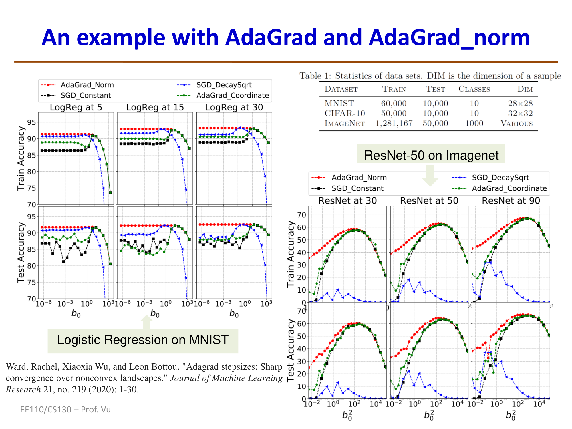
AdaGrad-norm Variant

AdaGrad-norm is a variant of AdaGrad. Instead of element-wise division, it divides only by the cumulative squared norm of the gradient vector (a scalar value):

AdaGrad-norm algorithm: Initialize learning rate \(\eta\), parameters \(\theta\), \(b_0 > 0\)

Additional steps:

• Compute the cumulative squared norm: \(b_t^2 \leftarrow b_{t-1}^2 + \|\hat{g}_t\|_2^2\) (scalar)
• Update parameters: \(\theta_t \leftarrow \theta_{t-1} - \eta \cdot \frac{\hat{g}_t}{b_t}\) (divide by the cumulative norm scalar)

Property: AdaGrad-norm has been proven to converge even for non-convex objective functions, i.e.:

\[ \min_{1 \le t \le T} \|\nabla J(\theta_t)\|^2 \le \epsilon_T \]

where \(\epsilon_T\) tends to zero at a rate of \(\frac{1}{\sqrt{T}}\). Convergence has been proven in both stochastic settings (convergence in probability) and deterministic settings (for \(T \ge N\)). (The only requirement is that \(J(\theta)\) is bounded below.)

RMSProp

RMSProp (Root Mean Square Propagation) was proposed by Geoffrey Hinton in his 2012 Coursera course (no formal paper was published). It is a direct fix for AdaGrad's monotonically decreasing learning rate problem.

Core idea: RMSProp replaces AdaGrad's cumulative sum of squared gradients with an exponential moving average (EMA) of squared gradients. This means the algorithm "forgets" distant historical gradients and focuses only on recent gradient information, thereby preventing the learning rate from shrinking to zero.

Derivation of the Exponential Moving Average (EMA)

Notice how AdaGrad aggressively reduces the effective step size by accumulating all historical gradients. One way to mitigate this is to gradually "forget" older gradient values, which leads to the exponential moving average (EMA) technique:

AdaGrad accumulation: \(\hat{v}_t \leftarrow \hat{v}_{t-1} + \hat{g}_t^2\)

EMA (i.e., RMSProp): \(\hat{v}_t \leftarrow \beta_t \hat{v}_{t-1} + (1 - \beta_t)\hat{g}_t^2\)

where \(\beta_t\) is the "forgetting factor" or weight factor.

Expanding the EMA recurrence (assuming constant \(\beta_t = \beta\)):

\[ v_t = \beta^t v_0 + \beta^{t-1}(1-\beta)g_1^2 + \beta^{t-2}(1-\beta)g_2^2 + \dots + \beta(1-\beta)g_{t-1}^2 + (1-\beta)g_t^2 \]

Since \(0 < \beta < 1\) and \(\beta^t \to 0\) as \(t\) increases, old gradient values are progressively down-weighted in the sum.

Algorithm formulation:

\[ v_t = \rho \cdot v_{t-1} + (1 - \rho) \cdot g_t^2 \]

\[ \theta_{t+1} = \theta_t - \frac{\eta}{\sqrt{v_t + \epsilon}} \cdot g_t \]

where \(\rho\) is the decay rate, typically set to \(0.9\) or \(0.99\). \(v_t\) is the exponential moving average of squared gradients.

Comparison with AdaGrad: In AdaGrad, \(G_t = \sum_{\tau=1}^{t} g_\tau^2\) is a simple cumulative sum of all historical squared gradients that can only increase. In contrast, \(v_t\) in RMSProp is a weighted average where the influence of old gradients decays exponentially (with an effective window size of approximately \(\frac{1}{1-\rho}\)). This prevents the effective learning rate from monotonically decreasing, allowing it to remain at a reasonable level even in the later stages of training.

Why it works: The name RMSProp comes from "Root Mean Square" — it takes the mean of recent squared gradients and then the square root. This value serves as an estimate of the typical magnitude of recent gradients. Normalizing the current gradient by this value makes the update step size for each parameter inversely proportional to the "typical size" of its recent gradients, thereby achieving adaptive learning rates.

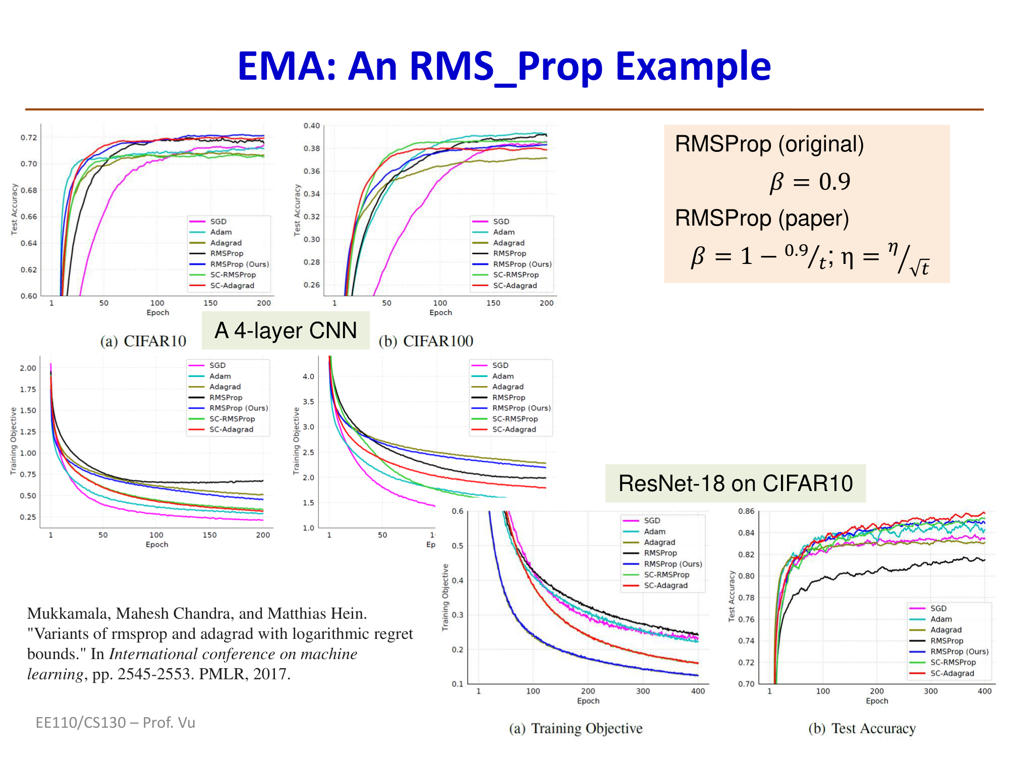
The original RMSProp (Hinton) recommends \(\beta_t = 0.9\) (constant). Some recent variants suggest adaptively adjusting \(\beta_t\), e.g., \(\beta_t = 1 - \frac{0.9}{t}\), while also adjusting the learning rate to \(\eta_t = \frac{\eta}{\sqrt{t}}\). These modifications can yield better convergence, but performance depends on the specific deep learning model and dataset complexity.

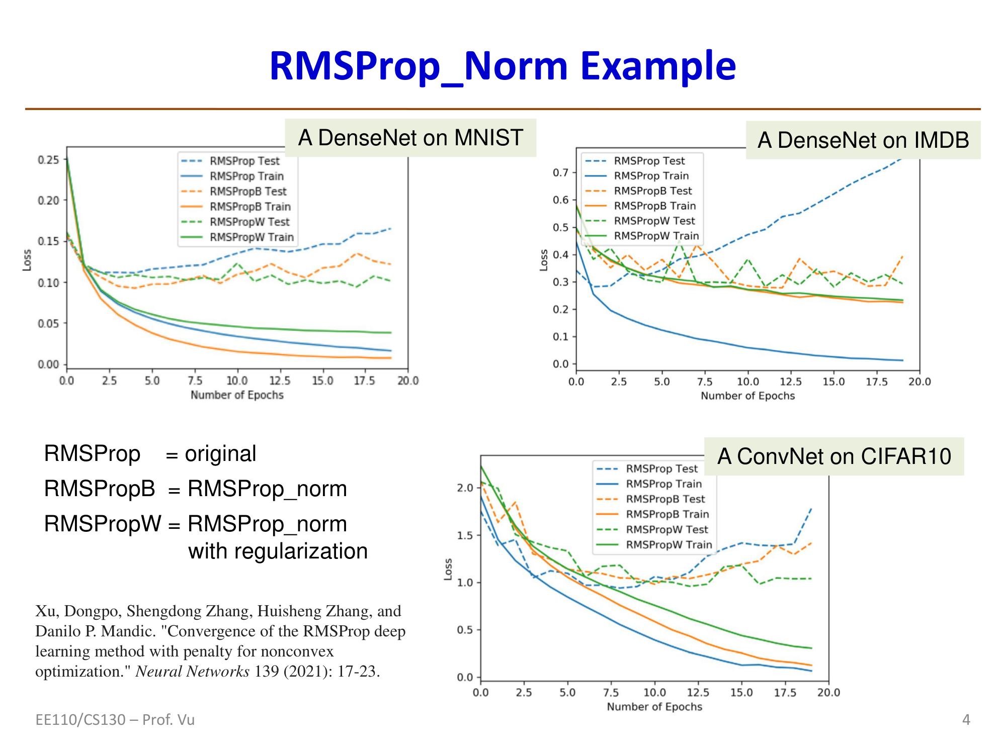
RMSProp-norm Variant

Similar to AdaGrad-norm, RMSProp also has a norm variant:

RMSProp (vector form): \(\hat{v}_t \leftarrow \beta\hat{v}_{t-1} + (1-\beta)\hat{g}_t^2\) (element-wise)

RMSProp-norm (scalar form): \(\hat{v}_t \leftarrow \beta\hat{v}_{t-1} + (1-\beta)\frac{\|g_t\|^2}{d}\) (scalar, where \(d\) is the dimension of \(g_t\))

Both share the same update rule: \(\theta_t \leftarrow \theta_{t-1} - \eta \cdot \frac{g_t}{\sqrt{v_t + \delta}}\)

RMSProp-norm also has guaranteed convergence for non-convex objective functions with a fixed step size (under mild conditions — bounded below).

AdaDelta

AdaDelta was proposed by Zeiler in 2012 as another fix for AdaGrad's decaying learning rate problem, developed independently and nearly simultaneously with RMSProp.

Key feature: AdaDelta not only uses an exponential moving average of squared gradients (similar to RMSProp) but also eliminates the need for an initial learning rate \(\eta\) altogether. It achieves this by additionally maintaining an EMA of squared parameter updates to automatically determine the update magnitude.

Algorithm formulation:

First, compute the EMA of squared gradients (same as RMSProp):

\[ v_t = \rho \cdot v_{t-1} + (1 - \rho) \cdot g_t^2 \]

Then compute the parameter update:

\[ \Delta \theta_t = - \frac{\sqrt{s_{t-1} + \epsilon}}{\sqrt{v_t + \epsilon}} \cdot g_t \]

Finally, update the EMA of squared parameter updates:

\[ s_t = \rho \cdot s_{t-1} + (1 - \rho) \cdot (\Delta \theta_t)^2 \]

\[ \theta_{t+1} = \theta_t + \Delta \theta_t \]

Note that \(\sqrt{s_{t-1} + \epsilon}\) in the numerator replaces the traditional learning rate \(\eta\) — it is automatically determined by the RMS of historical updates. This makes AdaDelta completely free of a manually set initial learning rate, eliminating one hyperparameter.

Practical usage: Although AdaDelta is theoretically elegant, Adam typically outperforms it in practice, so AdaDelta is used far less frequently than Adam and RMSProp.

---

Summary of Methods

Before moving on to Adam, let us review all the methods discussed so far:

Method	Required Hyperparameters	Update Rule	Key Feature
GD / SGD	Learning rate \(\eta\), initial point \(\theta^{(0)}\)	\(\theta^{t+1} = \theta^t - \eta g_t\)	Baseline method
AdaGrad	Learning rate \(\eta\), initial point \(\theta^{(0)}\)	\(v_t = v_{t-1} + g_t^2\); \(\theta^{t+1} = \theta^t - \eta\frac{g_t}{\sqrt{v_t+\epsilon}}\)	Accumulates squared gradients for adaptive search direction
RMSProp (EMA)	Learning rate \(\eta\), initial point \(\theta^{(0)}\), forgetting factor \(\beta\)	\(v_t = \beta v_{t-1} + (1-\beta)g_t^2\); \(\theta^{t+1} = \theta^t - \eta\frac{g_t}{\sqrt{v_t+\epsilon}}\)	Gradually forgets old gradient values
Polyak Momentum	Learning rate \(\eta\), momentum coefficient \(\mu\), 2 initial points \(\theta^{(0)}, \theta^{(1)}\)	\(m_t = \mu m_{t-1} - \eta g_t\); \(\theta^{t+1} = \theta^t + m_t\)	Introduces momentum term (first moment)
Nesterov (NAG)	Learning rate \(\eta\), momentum coefficient \(\mu\), 2 initial points \(\theta^{(0)}, \theta^{(1)}\)	\(m_t = \mu m_{t-1} - \eta g(\theta_t + \mu m_{t-1})\); \(\theta^{t+1} = \theta^t + m_t\)	Look-ahead gradient

---

Adam

Adam = Momentum + Adaptive Gradient

The Adam Optimizer

Adam (Adaptive Moment Estimation) was proposed by Kingma and Ba in 2015 (arXiv:1412.6980, 2014). It combines the core ideas from all previous methods:

• AdaGrad: Accumulates squared gradients (also called the "second moment")
• RMSProp: Exponential moving average
• Polyak: Introduces momentum (also called the "first moment") by accumulating gradients

Adam integrates all of these ideas into a single method.

Adam algorithm: Requires learning rate \(\eta\), momentum coefficient \(\mu\), two forgetting factors \(\beta_1, \beta_2\), two initial points \(\theta^{(0)}, \theta^{(1)}\)

\[ g_t \leftarrow \nabla J(\theta^t) \quad \text{(current gradient vector)} \]

\[ m_t \leftarrow \beta_1 m_{t-1} + (1 - \beta_1) g_t \quad \text{(EMA of the first moment)} \]

\[ v_t \leftarrow \beta_2 v_{t-1} + (1 - \beta_2) g_t^2 \quad \text{(EMA of the second moment)} \]

\[ \hat{m}_t \leftarrow \frac{m_t}{1 - \beta_1^t} \quad \text{(bias correction)} \]

\[ \hat{v}_t \leftarrow \frac{v_t}{1 - \beta_2^t} \quad \text{(bias correction)} \]

\[ \theta^{t+1} \leftarrow \theta^t - \eta \cdot \frac{\hat{m}_t}{\sqrt{\hat{v}_t} + \epsilon} \quad \text{(adaptive momentum update)} \]

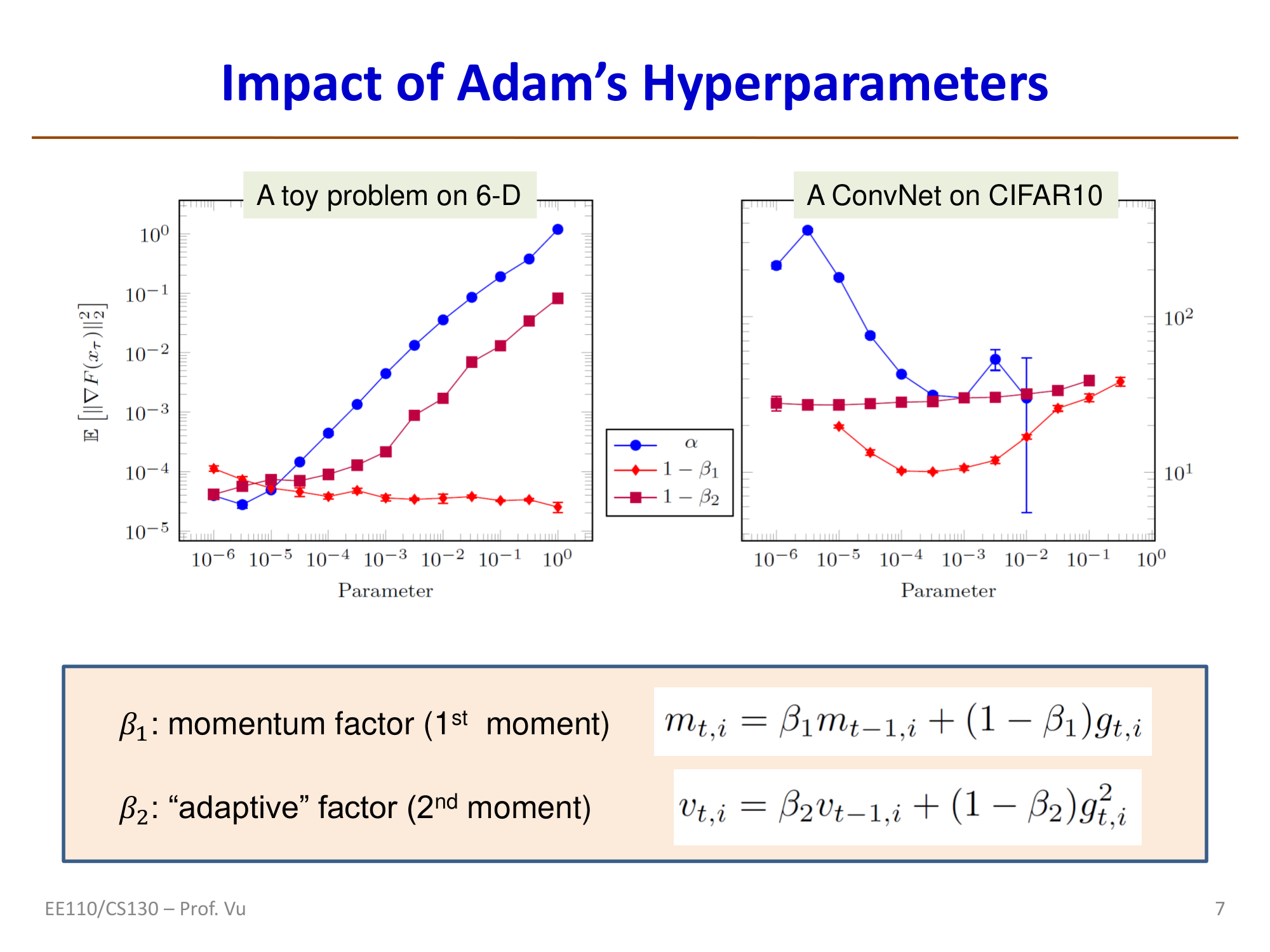
where \(\beta_1\) is the momentum factor (first moment) and \(\beta_2\) is the "adaptive" factor (second moment). The typical recommended values are \(\beta_1 = 0.9\) and \(\beta_2 = 0.999\) — very large (close to 1) momentum coefficients.

Mathematical Derivation of Bias Correction

Bias correction is the key innovation of Adam over simply combining Momentum and RMSProp. Let us derive the source of the bias using the second moment \(v_t\) as an example.

Starting from the recurrence with \(v_0 = 0\):

\[ v_1 \leftarrow (1 - \beta_2)g_1^2 \]

\[ v_2 \leftarrow \beta_2 v_1 + (1 - \beta_2)g_2^2 = \beta_2(1-\beta_2)g_1^2 + (1-\beta_2)g_2^2 \]

\[ v_3 \leftarrow \beta_2^2(1-\beta_2)g_1^2 + \beta_2(1-\beta_2)g_2^2 + (1-\beta_2)g_3^2 \]

In general:

\[ v_t = (1 - \beta_2)\sum_{i=1}^{t} \beta_2^{t-i} g_i^2 \]

Now consider that when training a DNN, \(g_t\) is stochastic, so \(v_t\) is also a random variable. Taking its expectation:

\[ \mathbb{E}[v_t] = (1 - \beta_2)\sum_{i=1}^{t} \beta_2^{t-i} \mathbb{E}[g_i^2] \]

Assuming \(\mathbb{E}[g_i^2] = \mathbb{E}[g_t^2]\) (the second moment of the gradient is the same at all steps):

\[ \mathbb{E}[v_t] = (1 - \beta_2) \cdot \frac{1 - \beta_2^t}{1 - \beta_2} \cdot \mathbb{E}[g_t^2] = (1 - \beta_2^t) \cdot \mathbb{E}[g_t^2] \]

Therefore:

\[ \mathbb{E}[g_t^2] = \frac{1}{1 - \beta_2^t} \mathbb{E}[v_t] \]

This \(\frac{1}{1 - \beta_2^t}\) is the bias correction factor. The bias arises from the EMA step — when initialized with \(v_0 = 0\), the early values of \(v_t\) are systematically biased downward. The corrected \(\hat{v}_t = \frac{v_t}{1-\beta_2^t}\) is an unbiased estimate of the true second moment \(\mathbb{E}[g_t^2]\). Similarly, \(\hat{m}_t = \frac{m_t}{1-\beta_1^t}\) is an unbiased estimate of the true first moment.

Impact of Adam Hyperparameters

Experiments show (see the figure below) that among Adam's three key hyperparameters:

• Learning rate \(\alpha\) (i.e., \(\eta\)) has the greatest impact on performance and requires careful tuning
• \(1 - \beta_1\) has the second-greatest impact
• \(1 - \beta_2\) has relatively little impact and is not very sensitive to its value

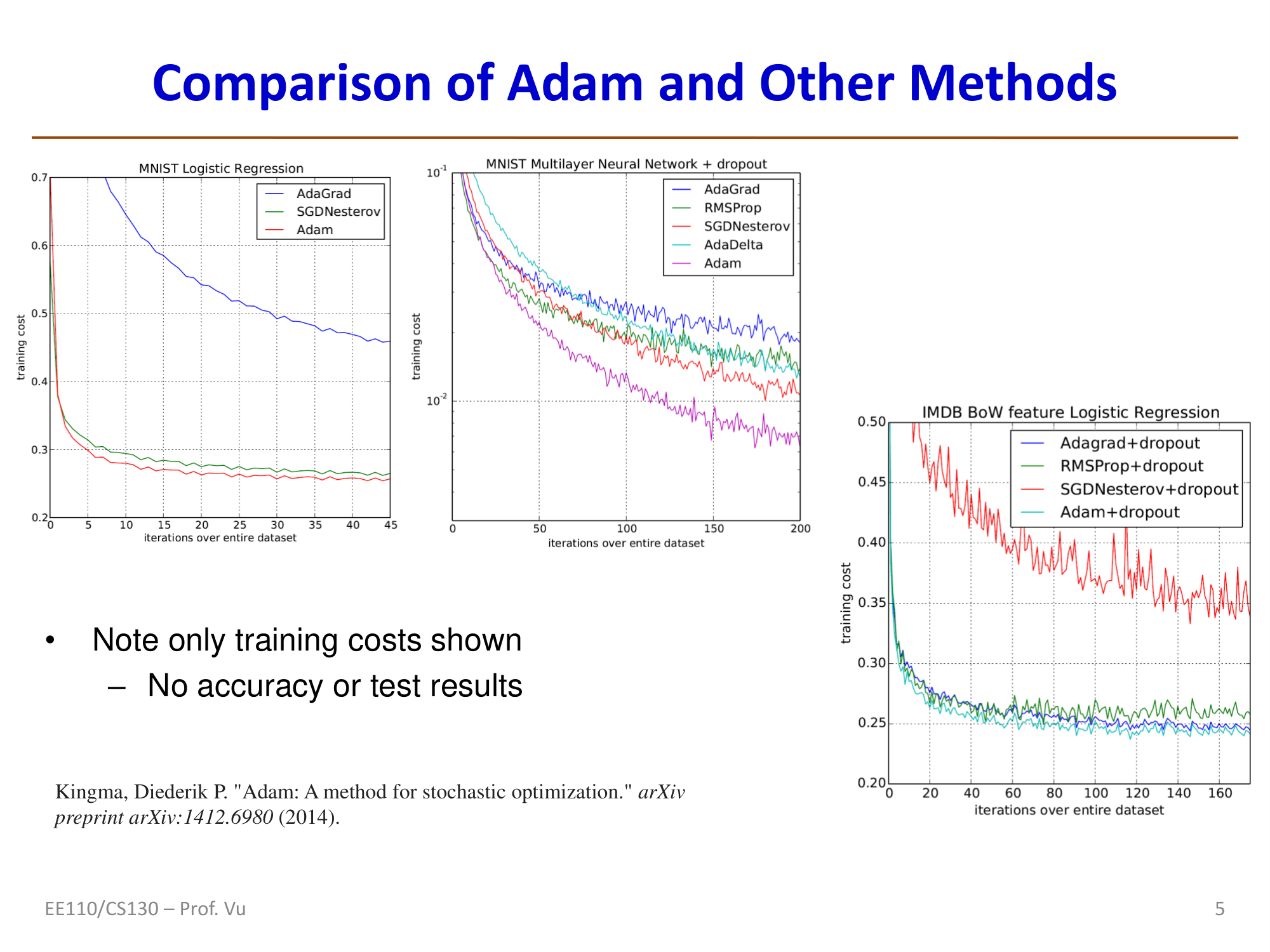
Comparison of Adam with Other Methods

The figure below shows a comparison of training cost between Adam and AdaGrad, SGDNesterov, RMSProp, and AdaDelta across different tasks (Kingma, 2014). Adam typically reduces training cost more quickly.

Convergence Properties of Adam

Convergence properties of Adam vs. AdaGrad (Defossez, 2022):

Method	Setting	Convergence Rate
Original AdaGrad	\(\beta_1 = 0\), fixed learning rate \(\eta\)	\(\mathbb{E}[\|g(\theta_N)\|^2] \sim O\left(\frac{1}{\sqrt{N}}\log N\right)\)
AdaGrad + adaptive LR	\(\eta_t = \frac{\eta}{t}\sqrt{\frac{1-\beta_2^t}{1-\beta_2}}\)	\(\mathbb{E}[\|g(\theta_N)\|^2] \sim O\left(\frac{1}{N}\right)\)
Adam + fixed LR	\(\beta_1 \ne 0\), \(\eta\) fixed	\(\mathbb{E}[\|g(\theta_N)\|^2] \sim O\left(\frac{1}{\sqrt{N}}\log N\right)\)
Adam + adaptive LR	\(\beta_1 \ne 0\), \(\eta_t = \eta(1-\beta_1)\sqrt{\frac{1-\beta_2^t}{1-\beta_2}}\)	\(\mathbb{E}[\|g(\theta_N)\|^2] \sim O\left(\frac{1}{N}\right)\)

Using an adaptive learning rate schedule can improve the convergence rate from \(O(\frac{1}{\sqrt{N}}\log N)\) to \(O(\frac{1}{N})\).

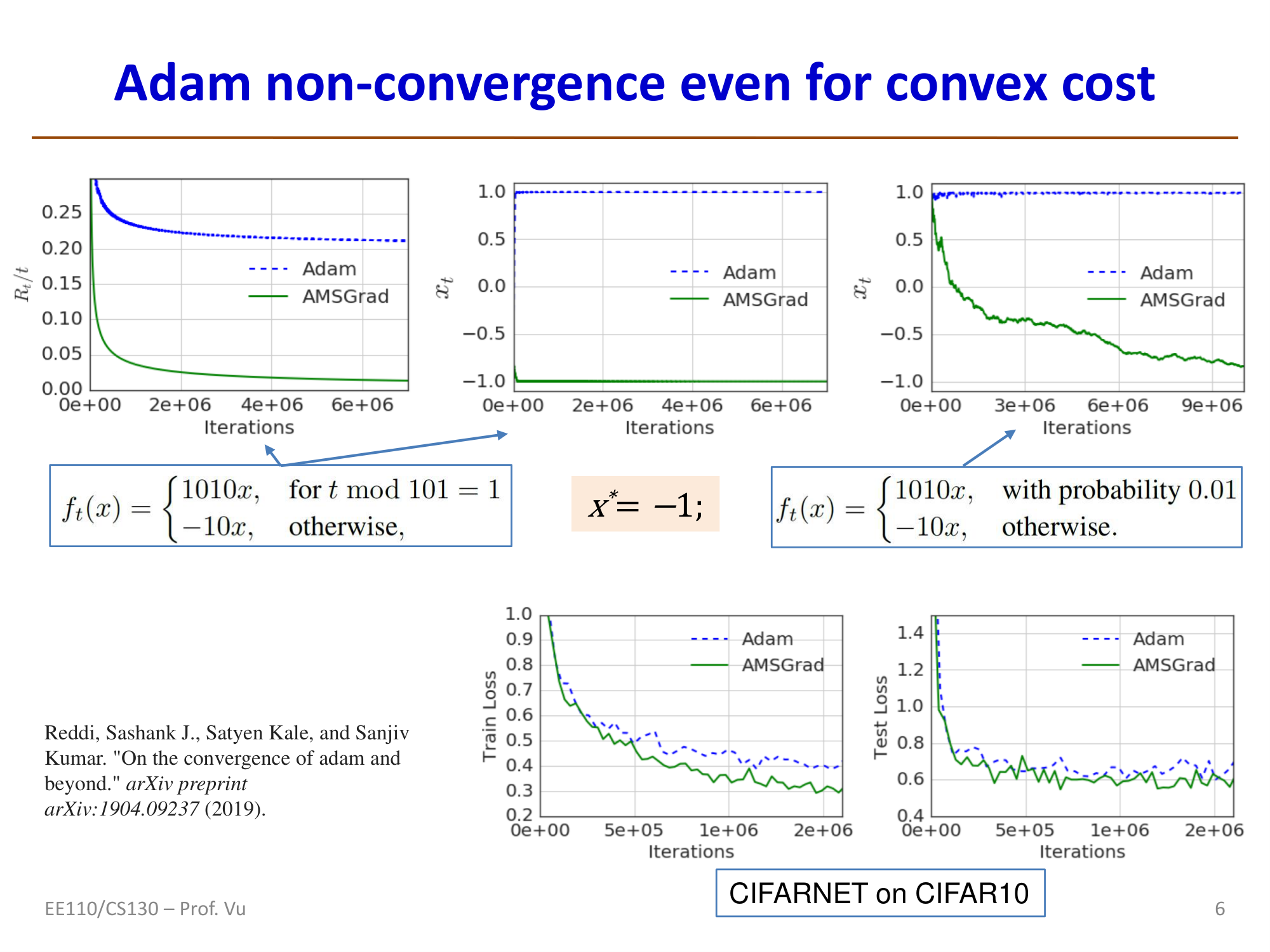
Non-convergence of Adam and AMSGrad

Adam may not converge (Reddi et al., 2019): even for convex objective functions, Adam can fail to converge. The root cause lies in the EMA step.

In non-EMA algorithms such as SGD and AdaGrad, the effective learning rate is monotonically non-increasing:

• For SGD (with adaptive learning rate \(\eta_t = \frac{\eta}{\sqrt{t}}\)): \(\gamma_t = \frac{1}{\eta_{t+1}} - \frac{1}{\eta_t} = \frac{1}{\eta}(\sqrt{t+1} - \sqrt{t}) > 0\)
• For AdaGrad (\(v_t = \sum_{i=1}^{t} g_i^2\)): \(\gamma_{t+1} = \frac{1}{\eta}\left(\sqrt{\sum_{i=1}^{t+1}g_i^2} - \sqrt{\sum_{i=1}^{t}g_i^2}\right) > 0\)

However, for EMA-based methods (RMSProp, Adam), the effective learning rate can increase, which may lead to non-convergence.

AMSGrad (a corrected version of Adam): The core idea is to retain the maximum of \(v_t\) seen so far:

\[ m_t \leftarrow \beta_1 m_{t-1} + (1 - \beta_1)g_t \]

\[ v_t \leftarrow \beta_2 v_{t-1} + (1 - \beta_2)g_t^2 \]

\[ \hat{v}_t \leftarrow \max(v_t, \hat{v}_{t-1}) \quad \text{(AMSGrad's new step: retain the maximum)} \]

\[ \hat{m}_t \leftarrow \frac{m_t}{1 - \beta_1^t} \quad \text{(bias correction)} \]

\[ \hat{v}_t \leftarrow \frac{\hat{v}_t}{1 - \beta_2^t} \quad \text{(bias correction)} \]

\[ \theta^{t+1} \leftarrow \theta^t - \eta \cdot \frac{\hat{m}_t}{\sqrt{\hat{v}_t} + \epsilon} \]

AMSGrad has been proven to guarantee convergence.

Adam Hyperparameter Considerations

Convergence proofs typically require:

• \(\beta_1 < \beta_2\), and \(\beta_1 < \sqrt{\beta_2}\) (stronger momentum on the second moment is desired since it involves \(g_t^2\))
• Learning rate schedule: \(\alpha_t = \frac{\alpha}{\sqrt{t}}\) or \(\eta_t = \frac{\eta}{\sqrt{t}}\)

Various convergence proofs exist for different hyperparameter regimes covering both convex and non-convex objectives (see Reddi 2018, Defossez 2022, Bock 2018, Zou 2019).

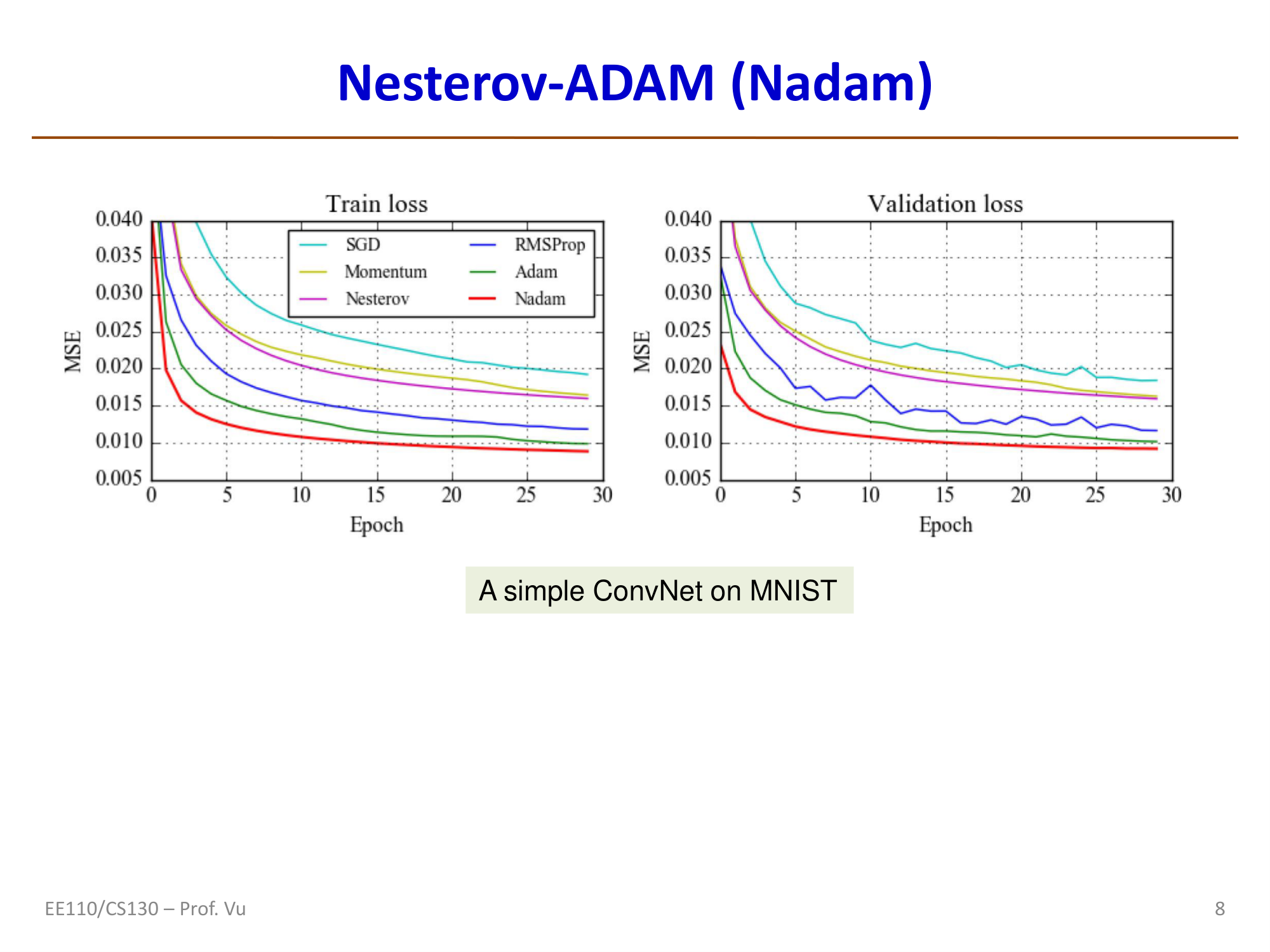
Nadam

Nadam (Nesterov-accelerated Adaptive Moment Estimation) was proposed by Dozat in 2016 and combines Adam with Nesterov momentum.

Motivation: Recall the Polyak momentum update:

\[ m_t \leftarrow \mu m_{t-1} - \eta g_t, \quad \theta^{t+1} \leftarrow \theta^t + m_t \]

Merging the two steps: \(\theta^{t+1} = \theta^t + (\mu m_{t-1} - \eta g_t)\)

In Polyak, \(g_t\) and \(m_{t-1}\) are independent. In Nesterov, \(g_t\) is made to depend on \(m_{t-1}\):

\[ g_t \leftarrow \nabla J(\theta_t + \mu m_{t-1}) \]

Nesterov vs. Nadam:

Nesterov	Nadam
\(g_t \leftarrow \nabla J(\theta_t + \mu m_{t-1})\)	\(g_t \leftarrow \nabla J(\theta_t)\)
\(m_t \leftarrow \mu m_{t-1} - \eta g_t\)	\(m_t \leftarrow \mu m_{t-1} - \eta g_t\)
\(\theta^{t+1} \leftarrow \theta^t + m_t\)	\(\theta^{t+1} \leftarrow \theta^t + (\mu m_t - \eta g_t)\)

Note that the two algorithms are not exactly the same. Nesterov applies the look-ahead at the gradient computation step, while Nadam applies the new momentum at the parameter update step.

Within the Adam framework, this changes the computation of the bias-corrected first moment \(\hat{m}_t\):

Adam: \(\hat{m}_t \leftarrow \frac{m_t}{1 - \beta_1^t}\)

Nadam: \(\hat{m}_t \leftarrow \frac{\beta_1 m_t}{1 - \beta_1^{t+1}} + \frac{(1-\beta_1)g_t}{1 - \beta_1^t}\)

AdamW

---

Second-Order Optimizers

Second-Order Optimizers have evolved chronologically as follows:

1. Pure Second-Order: Newton's Method (17th century), Quasi-Newton L-BFGS (1989)
2. Approximate Second-Order: KFAC (2015), AdaHessian (2020)

If SGD is first-order optimization (looking only at the current "slope"), then second-order optimization considers both the "slope" (gradient) and the "rate of change of the slope" (curvature).

Newton's Method

Newton's method is the foundation of second-order optimization. It approximates the objective function by expanding the Taylor series to second order. The core idea is to fit a quadratic surface to the objective function at the current point and directly jump to the minimum of that quadratic surface.

\[ \theta_{t+1} = \theta_t - H^{-1} \nabla f(\theta_t) \]

where \(H\) is the Hessian matrix (the matrix of second-order derivatives) and \(\nabla f\) is the gradient (first-order derivative).

AdaHessian

Since standard Newton's method is infeasible for deep learning, AdaHessian (An Adaptive Second-order Optimizer) is a popular recently proposed "approximate second-order optimizer." It aims to combine Adam's adaptivity with second-order curvature information. In certain complex tasks (such as Transformers or vision models), AdaHessian often achieves better generalization than Adam and is less sensitive to hyperparameters.

---

评论