Search and Optimization
The primary focus of classical artificial intelligence is making intelligent decisions within vast search spaces using general-purpose strategies.
Formal Definition
In computational theory, if you can reduce problem A to problem B, then solving B also solves A. Can we model any AI problem as a single class of problems, allowing convenient reductions similar to NP problems? AI pioneers Herbert Simon and Allen Newell developed the General Problem Solver (GPS) program in 1959. It was the first AI program in history that attempted to separate "search strategy" from "domain knowledge," aiming to simulate how humans approach problem-solving.
In AIMA, we can see that AI engineering practice transforms general problem solving into a form of constrained search. In other words, no matter how complex your problem is, if you want a computer to solve it, you must ultimately express it in the language of search. Put differently, given a sufficiently powerful modeling approach, there is no general problem that search cannot address. We refer to this search-based version of the general problem solver from AIMA as a problem-solving agent.
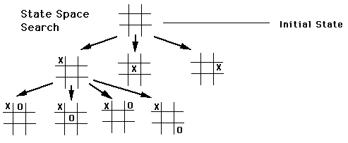
A problem-solving agent primarily solves state-space search problems, and its computational process is called search. In the discussions that follow, a search problem is synonymous with a general problem.
First, for any search problem, we must clearly define the states:
- State space, containing all possible environment states
- Initial state, the state in which the agent starts
- Goal state, one or more target states
Moving from the current position or any position to a goal position produces a path. Specifically:
- Path, a sequence of actions forming a route
- Solution, a path from the initial state to some goal state
We use the function \(g(n)\) to represent the total path length or total cost from the initial state to the current state \(n\). The AI compares \(g(n)\) values across different paths to find the most economical plan.
The fundamental building block for constructing path cost is the step cost function:
where:
- \(s\): the current state.
- \(a\): the action taken in that state.
- \(s'\): the new state resulting from taking the action.
We use path cost to refer to the sum of all step costs incurred from the initial state to the current node.
In a search problem, the AI's goal is typically to find a path from the initial state to the goal state that minimizes the total path cost \(g(n)\). In pseudocode, path cost is recorded as node.PATH-COST. It is computed cumulatively: child.PATH-COST = node.PATH-COST + action-cost. Best-first search (including UCS and A) records and compares this cumulative path cost* in the reached table to determine whether a better route has been found.
Additionally, the actions and action cost function are defined as:
- Action: given a state s, action(s) returns the set of executable actions
- Transition model: RESULT(s, a) returns the state that results from executing action a in state s
- Action cost function: ACTION-COST(s, a, s') gives the numerical cost of executing action a in state s, thereby transitioning to state s'
We assume that action costs are additive — that is, the total cost of a path is the sum of its individual action costs. An optimal solution is the solution with the lowest path cost among all solutions. For now, we assume all action costs are positive to reduce complexity.
The state space can be represented as a graph, where vertices represent states and directed edges between vertices represent actions.
This representational approach has persisted throughout AI's development. In reinforcement learning, this formulation is preserved. The idea of formalized search has never disappeared from AI. AlphaGo uses Monte Carlo Tree Search to look further ahead and employs neural networks to evaluate the winning probability of the current state, thereby guiding the search toward more promising directions. OpenAI's ChatGPT o1 chain-of-thought (CoT) is essentially finding solution paths in a reasoning space, using search to try multiple reasoning paths and backtracking upon failure to try alternatives.
Uninformed Search
In algorithm courses, we typically learn BFS and DFS — both of which are uninformed search methods.
Uninformed search only knows:
- The starting point
- The legal actions
- The goal
The limitation of uninformed search lies in its inefficiency. Since it performs no pruning and has no strategy, once the state space is large, the number of states to record and explore becomes enormous. Therefore, uninformed search can be viewed as a brute-force approach — its defining characteristic is that given sufficient time and space, it is guaranteed to find an answer.
An important note here: maintaining an explored set is merely an optimization technique used to convert "tree search" into "graph search."
Tree search means the algorithm treats the search space as an ever-expanding "tree" without caring whether a particular state (e.g., a specific puzzle configuration) has appeared before. Thus, if you go from A to B and then back to A, tree search treats the second A as a brand-new node and continues expanding it.
Graph search augments tree search with a "notebook" — the explored set. Whenever the algorithm finishes processing a node, it adds it to the explored set. When generating new nodes, the algorithm checks this record. If a state is already in the explored set (or still in the frontier waiting to be processed), it is discarded and not explored again. This ensures the algorithm never falls into the same trap twice, greatly improving efficiency and eliminating infinite loops.
BFS and Dijkstra
See the algorithm notes for details.
Bidirectional search is also based on BFS (breadth-first search), but it dramatically improves search efficiency by searching from both ends simultaneously.
Uniform-Cost Search
Breadth-first search assumes that each step has equal cost (e.g., all equal to 1). In the real world, different actions often have different costs (for example, taking the highway is faster but expensive, while taking back roads is slower but free). UCS handles such non-uniform cost scenarios and guarantees finding the lowest total cost optimal path.
The core idea of UCS is: always prioritize expanding the cheapest path.
DFS and Memory Issues
Backtracking search is a variant of DFS that uses less memory.
To prevent DFS from getting trapped in infinite paths, depth-limited search can be used.
Iterative deepening search follows a similar principle.
Heuristic Search
Heuristic search augments uninformed search with a heuristic function.
Heuristic Function
In the context of algorithms and AI, when we simply say "heuristic," we generally mean the heuristic function, written as h(n). The word originates from the Greek heuriskein (to discover).
We use g(n) to represent the actual cost and h(n) to represent the estimated cost from the current node n to the goal node. The evaluation function of a heuristic search must include at least h(n).
It is important to note that the heuristic function can "see" the board layout, but this layout is not the actual layout — rather, it is a predetermined, fixed layout. For example, in map navigation, the straight-line distance from a to b can serve as the heuristic function.
Admissibility
A heuristic function \(h(n)\) is said to be admissible if it satisfies one core condition: it never overestimates the actual minimum cost to reach the goal:
For any node \(n\), \(h^*(n)\) is the true minimum cost to reach the goal. This is an "optimistic" estimate — it assumes the remaining distance is at most this far, possibly closer, but never farther than the actual distance. An admissible heuristic guarantees finding the optimal solution (i.e., the solution with the lowest path cost) to the goal.
A heuristic function is consistent if it satisfies: for any node \(n\) and its successor \(n'\), the estimated cost from \(n\) to the goal is no greater than the sum of "the actual cost from \(n\) to \(n'\)" and "the estimated cost from \(n'\) to the goal":
This is analogous to the triangle inequality in geometry. As the path progresses, the estimated cost decreases no faster than the actual cost incurred. It is a sufficient condition for A* search on graph search to find the optimal solution without needing to revisit closed nodes.
For tree search, the heuristic must satisfy admissibility; for graph search, the heuristic must satisfy consistency.
Best-First Search
The core logic of best-first search is: always pick the node that "looks best" from the frontier for processing.
The algorithm works through two key data structures:
- Frontier: a priority queue ordered by the evaluation function \(f\). It ensures that each dequeued node has the smallest \(f(n)\) value (i.e., is deemed "best").
- Reached: a lookup table (hash table) that maps states to nodes. It is used not only for deduplication but also to store the lowest path cost for reaching each state.
The pseudocode is as follows:
BEST-FIRST-SEARCH
Starting node s
frontier: priority queue, initialized with starting node s, tracks the set of nodes currently being explored, sorted by evaluation function f
reached: lookup table, records distances from starting node s to other nodes, starting node s is also included (we may return to the starting node later)

While frontier is not empty:
    Pop node from frontier
    If node is the goal, end search, return node.
    If node is not the goal:
        Check what actions are available at node
        For each available action:
            successor state s' = RESULT(s, action)
            Compute cost from s to s' (path cost)
            If s' is not in reached, or this cost is less than the recorded cost:
                Update reached[s'] with this new node
                Add s' as a new node to the frontier queue

After the search ends, if no goal has been found, the search has failed, return Failure.
The significance of best-first search is that it provides a general algorithmic framework. By simply swapping the evaluation function \(f(n)\), it can switch between different search strategies to tackle different types of complex problems.
Its core value is: instead of blindly searching in a fixed order, it prioritizes the most promising nodes based on some criterion.
You can turn this general "framework" into specific familiar algorithms by adjusting the definition of \(f(n)\):
- f(n) = node depth → BFS
- f(n) = g(n) → Uniform-Cost Search (UCS)
- f(n) = g(n) + h(n) → A-Star
Greedy best-first search is also considered a heuristic search because it uses h(n).
A-Star
The A* algorithm is both complete and optimal.
The most classic application is the 8-Puzzle problem: the 8-Puzzle is a classic path search puzzle, typically consisting of a \(3 \times 3\) grid containing 8 numbered tiles (1–8) and one blank space.
The goal is to slide tiles to rearrange a scrambled initial state into a specific goal state (usually with numbers ordered 1 through 8 and the blank in the last position). You can only move tiles adjacent to the blank space into it, which visually appears as "moving the blank" in the four cardinal directions.
To make A* run faster while guaranteeing the minimum number of moves (optimal solution), the following two consistent heuristic functions are commonly used:
- Misplaced Tiles: Count how many tiles on the current board are not in their correct goal positions.
- Manhattan Distance: Compute the sum of the horizontal and vertical distances between each tile's current position and its goal position. This is the most commonly used heuristic — it is more "precise" than misplaced tiles and significantly reduces the number of nodes explored.
A search with a consistent heuristic is generally considered optimally efficient, because any algorithm that expands search paths from the initial state using the same heuristic information must expand all of A's necessarily expanded nodes. This efficiency also comes from pruning search tree nodes that do not help in finding the optimal solution.
Let us examine the following example:
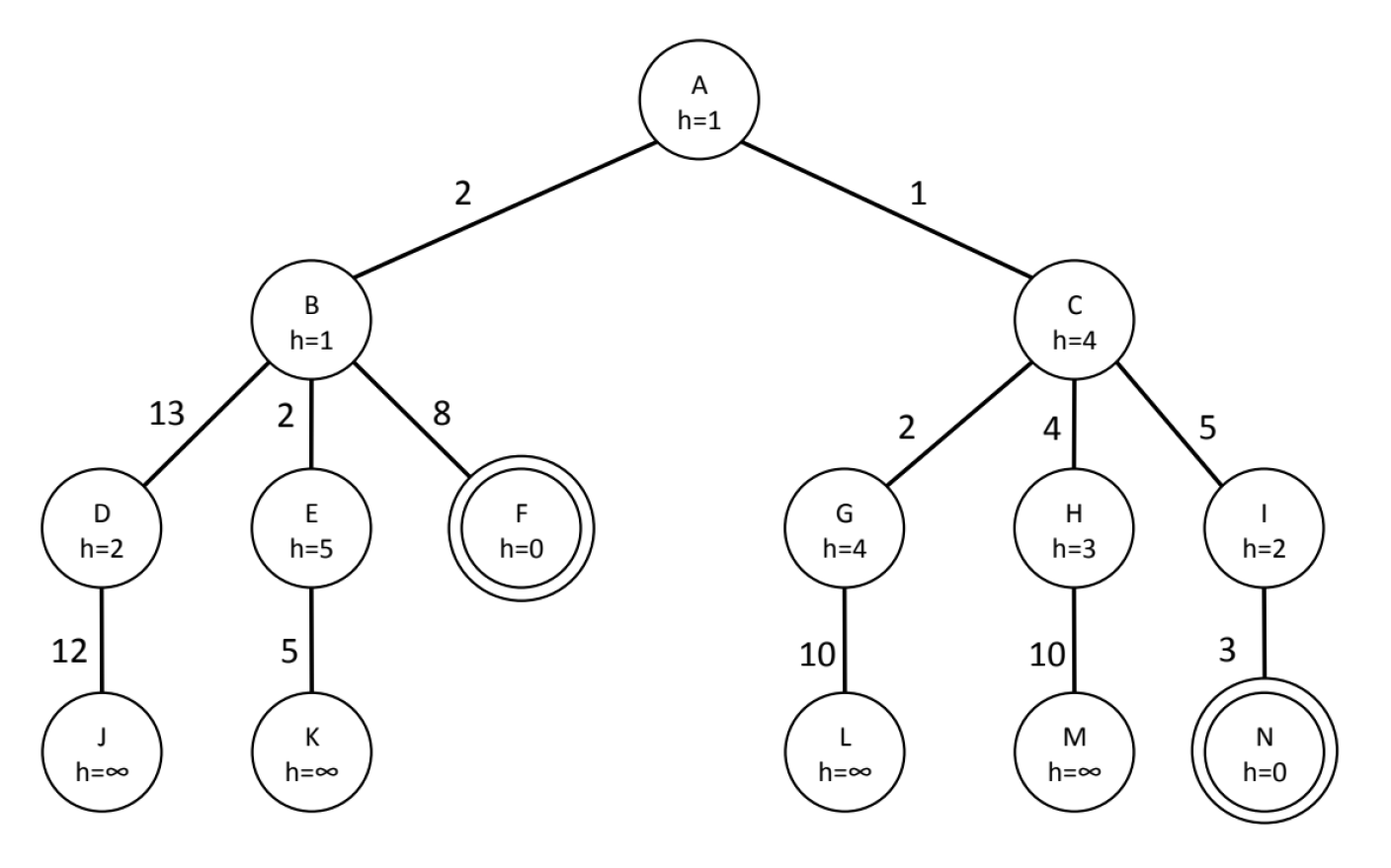
The \(h\) value (heuristic value) only represents the estimated distance from the current node to the goal — it is not cumulative. Therefore, when computing each node's \(f\) value (total evaluation score):
The core of the A algorithm is maintaining a priority queue, always selecting the node with the smallest \(f(n) = g(n) + h(n)\) for expansion*.
- \(g(n)\): the actual cost from the start node A to the current node.
- \(h(n)\): the heuristic estimate from the current node to the goal (the values inside the circles in the figure).
- Tie-breaking rule: if \(f\) values are equal, visit nodes in left-to-right order.
- Termination condition: when the goal node is expanded, the algorithm stops and returns the path.
We trace the state of the priority queue (open list / frontier) step by step:
Expand A: \(g(A)=0, h(A)=1 \Rightarrow f(A)=1\).
- Generate children: B and C.
- \(f(B) = g(B) + h(B) = 2 + 1 = 3\)
- \(f(C) = g(C) + h(C) = 1 + 4 = 5\)
- Queue: \([(B, f=3), (C, f=5)]\)
Expand B (since \(f=3\) is smallest):
- Generate children: D, E, F.
- \(f(D) = (2+13) + 2 = 17\)
- \(f(E) = (2+2) + 5 = 9\)
- \(f(F) = (2+8) + 0 = 10\)
- Queue: \([(C, f=5), (E, f=9), (F, f=10), (D, f=17)]\)
Expand C (since \(f=5\) is smallest):
- Generate children: G, H, I.
- \(f(G) = (1+2) + 4 = 7\)
- \(f(H) = (1+4) + 3 = 8\)
- \(f(I) = (1+5) + 2 = 8\)
- Queue: \([(G, f=7), (H, f=8), (I, f=8), (E, f=9), (F, f=10), (D, f=17)]\)
Expand G (since \(f=7\) is smallest):
- Generate children: L.
- \(f(L) = (1+2+10) + \infty = \infty\)
- Queue: \([(H, f=8), (I, f=8), (E, f=9), (F, f=10), (D, f=17), (L, f=\infty)]\)
Expand H (\(H\) and \(I\) both have \(f=8\); by the left-to-right rule, expand \(H\) first):
- Generate children: M.
- \(f(M) = (1+4+10) + \infty = \infty\)
- Queue: \([(I, f=8), (E, f=9), (F, f=10), (D, f=17), (L, f=\infty), (M, f=\infty)]\)
Expand I (since \(f=8\) is smallest):
- Generate children: N.
- \(f(N) = (1+5+3) + 0 = 9\)
- \(f(N) = (1+5+3) + 0 = 9\)
- Queue: \([(E, f=9), (N, f=9), (F, f=10), (D, f=17), \dots]\)
Expand E (\(E\) and \(N\) both have \(f=9\); by the left-to-right rule, expand \(E\) first):
- Generate children: K.
- \(f(K) = (2+2+5) + \infty = \infty\)
- Queue: \([(N, f=9), (F, f=10), (D, f=17), \dots]\)
Expand N (\(f=9\) is smallest. Since N is the goal node and is being expanded, the search terminates.)
Order of expanded nodes: A, B, C, G, H, I, E, N
The final path returned by the algorithm is the backtracking from the expanded goal node N to the start:
- N's parent is I
- I's parent is C
- C's parent is A
Final path: A \(\rightarrow\) C \(\rightarrow\) I \(\rightarrow\) N
The total cost of the final path is \(g(N)\):
- \(Cost(A, C) = 1\)
- \(Cost(C, I) = 5\)
- \(Cost(I, N) = 3\)
- Total cost: \(1 + 5 + 3 = 9\)
IDA*
Sliding Puzzle (N-Puzzle)
The sliding puzzle (N-Puzzle) is the "fruit fly" of the algorithm world — by studying it, we can glimpse the entire evolutionary history of search algorithms from simple to complex.
| Scale | Alias | State Space | Objective | Best Algorithm | Key Heuristic | Difficulty |
|---|---|---|---|---|---|---|
| \(2 \times 3\) | LeetCode 773 | 720 | Optimal solution | BFS | None needed (or Manhattan) | Entry-level |
| \(3 \times 3\) | 8-Puzzle | 180,000 | Optimal solution | A* | Manhattan distance | Easy |
| \(4 \times 4\) | 15-Puzzle | 10 trillion | Optimal solution | IDA* | Manhattan + Linear Conflict | Intermediate |
| \(5 \times 5\) | 24-Puzzle | \(10^{25}\) | Optimal solution | IDA* | Pattern Databases (PDB) | Hard |
| \(6 \times 6\) | 35-Puzzle | \(10^{41}\) | Feasible solution | Weighted A* / Greedy | Disjoint PDB / Deep Learning | Extreme (NP-Hard) |
Local Search
Local search is a heuristic algorithm used to solve combinatorial optimization problems. Simply put, its core idea is "take it one step at a time, always choosing a better option." The algorithm starts from an initial solution and iteratively improves it by searching for better solutions among the current solution's "neighbors," until it reaches a locally optimal state or a stopping condition is met.
Although in principle local search cannot find the global optimum and may get trapped at a local optimum, it is often "good enough" and sufficient for solving many problems where finding a global optimum is infeasible. Moreover, local search commonly serves as the "inner engine" of many advanced algorithms. Its extremely fast search speed is leveraged alongside various mechanisms for "escaping traps."
Hill Climbing
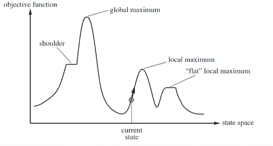
Consider the following state space landscape:
Hill climbing is a greedy algorithm with extremely simple logic:
- Start at a random point: randomly select a point as the initial position.
- Look around: examine the neighboring points (the neighborhood) near the current position.
- Move upward: if there is a point higher (better) than the current one, move to it.
- Stop at the peak: if all surrounding points are lower than the current one, assume the peak has been reached and stop searching.
Because hill climbing is myopic and never backtracks, it frequently encounters three awkward situations:
- Local maxima: It climbs to the top of a small hill. Although it is not the highest peak of the entire landscape, since everything around it slopes downward, it mistakenly believes it has reached the summit.
- Plateaus: The surrounding area is completely flat. The algorithm finds that every direction yields the same value, loses its sense of direction, and can only wander randomly (random walk).
- Ridges: This is a particularly interesting phenomenon. A ridge is narrow and steep; if you can only move along the cardinal directions (north-south or east-west), each step may be going downhill, causing the algorithm to oscillate between the two sides of the ridge without being able to follow the ridgeline upward.
Hill climbing by itself is not a particularly good algorithm, but it serves as a foundation for extending into practical algorithmic approaches.
Stochastic hill climbing introduces a stochastic element: among all uphill moves, one is chosen at random rather than always selecting the steepest. This gives it some probability of avoiding narrow local peaks. Here, the exploration vs. exploitation tradeoff emerges — a concept that becomes particularly important in reinforcement learning.
Building on stochasticity, random-restart hill climbing is the most practical variant of hill climbing. After reaching a peak, the algorithm teleports to another random starting point and climbs again. Given enough restarts, the probability of finding the global maximum becomes very high.
Min-Conflicts
N-Queens (Feasible Solution)
In the 8-Queens problem, a "state" is a complete arrangement of 8 queens on the board. We can easily define the neighborhood: moving one queen to a different row within the same column. The 8-Queens problem has a very intuitive evaluation function \(h\): the number of pairs of queens that are mutually attacking each other. Our goal is to minimize this \(h\) (which can be thought of as descending to the lowest elevation, i.e., "going downhill").
Random-restart hill climbing is probabilistically complete. Given enough restarts, it can almost certainly find a solution to the 8-Queens problem (since the state space is finite). Its efficiency depends on the density of "solution states" among all states. For the 8-Queens problem (8×8), it is fast; but for 8,000 queens, the blindness of random restarts becomes apparent.
In the 8-Queens (and all N-Queens) problem domain, min-conflicts heuristic is generally considered closer to the "optimal local search solution" than any form of hill climbing:
- Random-restart hill climbing: each attempt may need to evaluate all possible moves for all queens, choosing the best one (high computational cost).
- Min-Conflicts: randomly selects one conflicting queen, then finds only the position with the fewest conflicts for that queen.
- Empirical data: for the 1,000,000-Queens problem, random-restart hill climbing may still be repeatedly resetting the board, while Min-Conflicts typically converges to a solution within 50 steps.
| Range of N | Best Algorithm | Core Logic | Time |
|---|---|---|---|
| \(N \le 20\) | Standard backtracking | Ordinary DFS can find a solution. | Milliseconds |
| \(20 < N \le 10^4\) | Local search (Min-Conflicts) | A variant of hill climbing. Place queens randomly first, then repeatedly move the most conflicting queen. | Seconds (very fast) |
| \(N > 10^4\) | Mathematical construction | Use mathematical formulas to directly compute coordinates (e.g., patterns based on \(N \pmod 6\)). | \(O(N)\) milliseconds |
Note that if the goal is to find all solutions, the situation is entirely different — backtracking with bitwise operations is required, and for N >= 20 there is no known best algorithm. Current supercomputers can handle at most N = 27.
Metaheuristic Algorithms
The core of metaheuristic algorithms lies in managing the tension between exploration and exploitation:
- Global search (exploration)
- Local refinement (exploitation)
Metaheuristics dynamically adjust the balance between these two through some mechanism (such as the temperature in simulated annealing or mutation in genetic algorithms), enabling the algorithm to escape local optima and move toward the global optimum.
Common metaheuristic algorithms include:
- Simulated Annealing (SA): allows accepting "worse" solutions with some probability, providing opportunities to escape local traps.
- Tabu Search: builds a "tabu list" to prevent the algorithm from repeatedly revisiting recently explored areas.
- Variable Neighborhood Search: when no better solution can be found in one neighborhood, the search scope is expanded by changing the neighborhood definition.
- Evolutionary algorithms
- Particle swarm optimization
- Ant colony optimization
Simulated Annealing
Simulated annealing (SA) is a probabilistic global optimization algorithm inspired by physics. Its core intuition comes from the annealing process in metallurgy: when a solid is heated to high temperature and then slowly cooled, its particles gradually settle into stable low-energy states as the temperature drops, ultimately forming a perfect crystal (i.e., the global optimum). The core purpose of simulated annealing is to solve the "local optimum" trap. Traditional hill climbing (greedy search) only moves in improving directions and easily gets stuck on a hillside. SA allows moving in worse directions with some probability, thereby jumping out of local traps.
The simulated annealing algorithm generally proceeds through the following steps:
- Starting from the current state, the algorithm randomly selects a neighboring state (called a successor). This randomness is the foundation of SA's ability to explore different possibilities, rather than rigidly moving in a single direction.
- If the randomly generated successor is better than the current state, the algorithm moves to the new state with 100% certainty — i.e., the algorithm always accepts good moves.
- If the randomly generated successor is worse than the current state, the algorithm accepts it with some probability — i.e., the algorithm accepts worse moves with a certain probability. This probability generally follows the Boltzmann distribution.
- Over time, the probability of accepting worse moves is gradually reduced. The key variable controlling this is the temperature.
In simple terms, during the initial phase (analogous to high temperature), the algorithm is very "wild" — the probability of accepting bad moves is high, with the purpose of broadly exploring a wide area. In the later phase (analogous to low temperature), the algorithm becomes increasingly conservative — the probability of accepting bad moves gradually decreases until it stabilizes, locking in on the best region it has discovered.
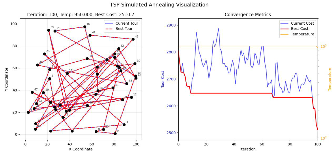
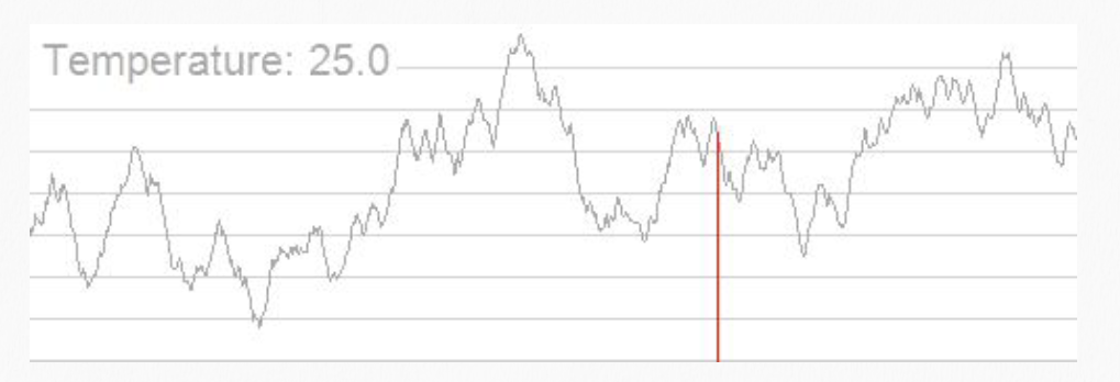
In the figure above, when simulated annealing is applied to the Traveling Salesman Problem (TSP), the route appears very chaotic (left panel), indicating that the algorithm is performing "broad-range exploration." In the right panel, the blue line fluctuates wildly and the temperature (yellow line) is high — the algorithm is deliberately accepting worse routes.
A note on terminology: in the TSP context, "cost" refers to the objective function value that the algorithm tries to minimize. Generally, cost refers to the total physical distance the salesman travels to visit all cities and return to the starting point. Lower cost indicates a better route; higher cost indicates a more circuitous, less efficient path.
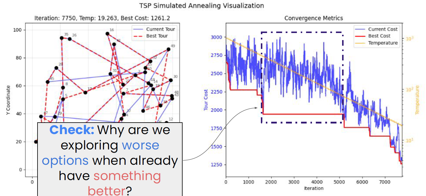
In the figure above, the route has become much clearer, and the red dashed line represents the best path found so far (left panel). Notice the dashed box in the right panel: although the red line (best cost) has dropped below 2,000, the blue line is still jumping significantly between 2,000 and 3,000. We still need to explore worse solutions because between iterations 2,000 and 5,000, the algorithm may have been stuck in a local optimum. If the blue line were not allowed to jump upward (accept worse solutions), it would never be able to cross the barrier to discover the lower, better red plateau after iteration 5,000. As the temperature decreases in later stages, the blue line's fluctuation amplitude shrinks, eventually tracking the red line closely and locking in near the optimal solution.
The core mathematical logic of simulated annealing is the Boltzmann distribution and the Metropolis criterion.
Assume the current solution is \(x_{current}\) and a new solution \(x_{next}\) has been generated, with the energy (objective function value) difference \(\Delta E = f(x_{next}) - f(x_{current})\):
- If \(\Delta E < 0\) (the solution improved): accept the new solution with 100% probability.
- If \(\Delta E > 0\) (the solution worsened): accept the new solution with probability \(P\).
The probability \(P\) is computed as:
where \(T\) is the current "temperature":
- High temperature phase: \(P\) approaches 1. The algorithm traverses the search space almost like a random walk, with the goal of exploring globally.
- Low temperature phase: \(P\) approaches 0. The algorithm becomes very "conservative," accepting only better solutions, with the goal of fine-grained convergence.
The Metropolis criterion is the decision-making brain of simulated annealing, determining whether the algorithm accepts a "worsened" solution. Assume the current energy is \(E_{curr}\), the newly generated energy is \(E_{next}\), and the change is \(\Delta E = E_{next} - E_{curr}\).
The probability \(P\) of accepting the new solution is:
Note: in algorithmic practice, the Boltzmann constant \(k\) is typically set to 1 for simplicity.
This criterion originates from statistical mechanics. In a constant-temperature system, the probability of a particle being in a state with energy \(E\) follows the Boltzmann distribution. The Metropolis criterion simulates this natural equilibrium process: even though the system tends toward low-energy states, at a given temperature, particles still have some probability of jumping to higher-energy states.
The pseudocode for simulated annealing is as follows:
Algorithm: Simulated Annealing for TSP
-------------------------------------------------------

1.  [Initialization Phase]
    - Read the map: store all city coordinates in the CITIES array (e.g., CITIES[0] = [x0, y0])
    - Generate initial solution: CURRENT_TOUR = [0, 1, 2, ..., N-1] (randomly shuffled)
    - Compute cost: CURRENT_COST = compute_total_distance(CURRENT_TOUR)
    - Record best: BEST_TOUR = CURRENT_TOUR, BEST_COST = CURRENT_COST
    - Set initial parameters: temperature T = 1000, cooling rate ALPHA = 0.995, termination temperature = 0.01

2.  [Iterative Search Phase]
    While temperature T > termination temperature:

        Execute the following "perturbation" steps (typically repeated L times at each temperature):

        A. Perturbation:
           - Randomly select two positions: i, j = random_index(0, N-1)
           - Copy current path: NEW_TOUR = CURRENT_TOUR.copy()
           - Swap city indices: swap NEW_TOUR[i] and NEW_TOUR[j]

        B. Compute cost:
           - NEW_COST = compute_total_distance(NEW_TOUR)
           - Compute difference: DELTA_E = NEW_COST - CURRENT_COST

        C. Accept or reject:
           - If DELTA_E < 0 (new path is shorter):
               - CURRENT_TOUR = NEW_TOUR
               - CURRENT_COST = NEW_COST
               - If NEW_COST < BEST_COST (new historical best found):
                   - BEST_TOUR = NEW_TOUR
                   - BEST_COST = NEW_COST
           - Else (new path is longer):
               - Compute acceptance probability: P = exp(-DELTA_E / T)
               - If random(0, 1) < P:
                   - CURRENT_TOUR = NEW_TOUR  <-- probabilistically accept a "bad route"
                   - CURRENT_COST = NEW_COST

    3.  [Cooling Phase]
        - Update temperature: T = T * ALPHA

4.  [Termination Phase]
    - Output BEST_TOUR and BEST_COST
Python code can be found in the folder containing these notes (includes visualization of the process):
In practice, several common questions arise:
(1) How is the map stored?
Typically we use either a coordinate matrix or a distance matrix (more advanced).
A coordinate matrix stores an \(N \times 2\) list (or array) recording each city's \((x, y)\) coordinates. For example, cities = [[0, 0], [10, 5], [2, 8]]. Each time the Cost between two cities is computed, the Euclidean distance formula is used: \(\sqrt{(x_1-x_2)^2 + (y_1-y_2)^2}\).
A distance matrix pre-computes an \(N \times N\) table to avoid redundant calculations. dist[i][j] directly represents the distance from city \(i\) to city \(j\).
(2) How is the current state recorded?
Since simulated annealing is not completely blind random search but rather random perturbation based on the current position, each new path is always attempted from the current position. So how do we store the current position?
We do not need a single variable to record "where we currently are." Instead, we use an array to record the current visitation order. This array is the sole object the algorithm operates on.
Suppose there are 5 cities (indexed 0, 1, 2, 3, 4):
- Current_Tour (current path):
[0, 3, 1, 4, 2]This represents the salesman's route: 0 \(\to\) 3 \(\to\) 1 \(\to\) 4 \(\to\) 2 \(\to\) back to 0. - Best_Tour (historical best):
[0, 1, 2, 3, 4]This is the shortest path found so far.
If position swapping is used as the perturbation, it simply changes the arrangement of numbers in the array. For example, from [0, 3, 2, 1] to [0, 1, 2, 3].
(3) Specifics of computing cost
When computing total distance, remember that the last city must connect back to the first:
(4) Key variables
At any moment during execution, the main variables stored in memory are:
| Variable Name | Type | Purpose |
|---|---|---|
cities |
Matrix | The fixed map storing all city coordinates. |
current_tour |
Array | Core variable. Records the current city ordering (e.g., [2, 0, 1, 3]). |
new_tour |
Array | Temporary variable. A copy of current_tour with two randomly swapped points. |
best_tour |
Array | Safety net. Always stores the shortest arrangement found; unaffected by "bad solutions." |
T |
Float | Current temperature. Controls our "boldness" in accepting new_tour. |
.
Evolutionary Algorithms
Evolutionary algorithms (EA) do not rely on human logic to "design" solutions. Instead, they simulate Darwinian evolution, letting programs evolve optimal solutions through "survival of the fittest."
Evolutionary algorithms treat each possible solution to the problem as an "individual" and perform the following operations:
- Selection: like "natural selection." The algorithm evaluates the fitness of all current solutions; better-performing solutions have a greater chance of producing "offspring."
- Reproduction/Crossover: two good solutions exchange parts of their "genes" (subsets of parameters) to synthesize a new solution. As the slides state: combining two good states is likely to produce an even better state.
- Mutation: to prevent the algorithm from getting stuck in a local optimum (dead end), it randomly alters certain parts of a solution. This is akin to genetic mutation in biology — sometimes yielding unexpected breakthroughs.

The figure above shows one of the most classic applications of evolutionary algorithms: the NASA ST5 spacecraft antenna. Human engineers typically design regular geometric shapes (such as circular or rod-shaped antennas), but the computer completely disregards "aesthetics" or "symmetry" — it only optimizes for maximum signal gain through millions of simulated evolutionary iterations. The result is this bizarre shape that looks like a twisted paperclip. This seemingly chaotic design far outperforms any conventional antenna designed by top human experts.
Genetic Algorithms
Genetic algorithms (GA) are a specific implementation of evolutionary algorithms. Unlike evolutionary algorithms' emphasis on mutation and natural selection, GA places heavy emphasis on the crossover operation.
Genetic algorithms are best applied in scenarios where no explicit mathematical formula exists — such as the antenna mentioned above, or optimizing aircraft wing shapes. In these scenarios, one can only perform simulation-based testing.
For the 8-Queens problem, backtracking is the fastest approach; for larger N (e.g., N = 1000) where backtracking becomes infeasible, the optimal method is local search. Therefore, genetic algorithms are not the optimal algorithm for the 8-Queens problem.
The fitness function is a core component of evolutionary algorithms (such as genetic algorithms, genetic programming, etc.). Simply put, the fitness function is a "scorer" that measures how "good" a candidate solution (individual) is at solving the target problem.
For example, in the Unbounded Knapsack Problem (UKP), since each item can be selected an unlimited number of times, the fitness function design must consider not only how to maximize value but also how to elegantly handle "overweight" scenarios.
The most straightforward fitness measure is the total value of items in the knapsack. Suppose you select \(n\) types of items, where each item type has value \(v_i\) and selected quantity \(x_i\). The raw fitness is:
The penalty function addresses constraint violations. Again using the unbounded knapsack problem as an example, the only hard constraint is that the total weight cannot exceed the knapsack capacity \(W\). If a solution is overweight, we cannot simply discard it (because its genes may contain excellent fragments), but we must penalize its score. Two penalty strategies are available:
Approach A: Linear Penalty (Recommended)
If the total weight \(\sum (w_i \cdot x_i) > W\), deduct the cost of the excess weight from the total value.
Note: the coefficient \(\alpha\) must be large enough to ensure that overweight individuals score far below non-overweight ones. A common choice is the maximum value-to-weight ratio among all items (i.e., \(\max(v_i/w_i)\)).
Approach B: Death Penalty (Simple but less effective)
If overweight, the fitness is set directly to 0 or an extremely small negative number.
- Drawback: in the early stages of evolution, if all randomly generated solutions are overweight, the algorithm will devolve into blind search because it cannot find "relatively good" failed solutions to compare.
Traveling Salesman Problem (TSP)
Tribe-level perspective: evolutionary algorithms are at the core of the Evolutionaries tribe in Domingos's taxonomy. For full GA derivations (Schema theorem / selection operators / SBX crossover / tree-based GP), CMA-ES, NEAT neuroevolution, PSO/ACO, and AutoML/NAS, see The Master Algorithm — Evolutionaries.
Constraint Satisfaction Problems (CSP)
CSP Modeling
CSP modeling revolves around three core elements, typically represented as a triple \((X, D, C)\).
To model a problem as a CSP, the following three components must be clearly defined:
- Variable set \(X\) (Variables):
- Definition: \(X = \{X_1, X_2, \dots, X_n\}\) — the objects you need to solve for.
- Domain set \(D\) (Domains):
- Definition: \(D = \{D_1, D_2, \dots, D_n\}\) — each variable \(X_i\) has a corresponding range of possible values \(D_i\).
- Constraint set \(C\) (Constraints):
- Definition: \(C = \{C_1, C_2, \dots, C_m\}\) — describes the relationships that must hold between variables.
- Each constraint consists of a subset of variables and a permitted relation (i.e., legal assignment combinations).
- Constraints are ideally unary. A unary constraint involves only a single variable.