CNN

From MLP to CNN

Why Not Use MLP?

Building upon MLP, we now turn to CNN. For image processing tasks, MLP has an inherent flaw: the number of parameters in a single layer is prohibitively large. Suppose an image has 1M pixels — the input dimension would be 1M. If we use 1000 neurons, the total parameter count is:

• Input dimension: 1 million
• Output dimension: 1000

Total parameters = 1 million x 1000 + 1000 ≈ 1 billion.

Deep learning typically uses float32 (single-precision floating point), where each parameter takes 4 Bytes. Multiplying 1 billion by 4 bytes gives approximately 4GB. This is the weight size of just a single layer — with 10 layers, the weights alone would require 40GB of GPU memory, which is clearly unacceptable.

In summary, while the Universal Approximation Theorem guarantees that MLPs can capture features and learn to recognize images, the overly unconstrained architecture of MLPs causes the model to attempt learning all possible features. This means the model not only learns the shape of a cat but also attends to various noise patterns. Moreover, without the guidance of locality, searching for the optimal solution in the vast parameter space is like finding a needle in a haystack.

Therefore, the essential difference between CNN and MLP lies not in the ability to find features, but in parameter efficiency. We can think of CNN as a special, constrained form of MLP: it essentially zeros out most positions in the MLP weight matrix and forces the remaining non-zero positions to share the same values. This parameter reduction brings a tremendous advantage — it lays the foundation for stacking more layers, making deep networks practically feasible.

Core Assumptions

Beyond the excessive parameter issue of MLPs discussed above, we must introduce another critical problem: spatial structure. MLPs require flattening an image into a vector. For a fully connected layer, different pixels have no relationship — they are treated as entirely equal.

Based on these considerations, the Convolutional Neural Network architecture was proposed.

CNN rests on two fundamental assumptions:

1. A pixel is most closely related to its neighboring pixels (Locality)
2. A cat that moves from the top-left corner to the bottom-right corner is still a cat (Translation Invariance)

These prior assumptions are the two core inductive biases of CNN. One could even say the CNN architecture itself was invented to hard-code these two biases into mathematical formulas. These two key assumptions are the primary reason CNNs outperform MLPs on visual recognition tasks.

In addition, images possess other important properties:

• Size Invariance: Certain responses should be independent of the target's size
• Rotation Invariance: For example, a pencil remains a pencil after rotation
• Long-range Features: Higher-level visual features span longer distances and are typically captured only after lower-level feature detection

From these properties, CNN has three design motivations:

1. Sparse Interactions: Information is extracted from local image regions rather than through full connections
2. Parameter Sharing: The same set of parameters is used to process different image regions
3. Equivariant Representations: Visual signals at different positions are extracted in the same manner

Regarding inductive bias: "induction" refers to deriving general rules from specific instances — for example, if you look at 10,000 photos of cats and find they are all white, you might conclude that cats are white; "bias" refers to a tendency or preset constraint — for example, requiring a dating partner to be at least 180cm tall is a bias. An inductive bias is a constraint or preference we impose on a model in advance so that it can more effectively learn patterns from limited experience (induction).

Without such biases, given the same dataset, a model would become a student who merely memorizes by rote.

In the current era of large models, ViT has fewer biases than CNN but can capture more complex and flexible features, thus achieving a higher ceiling than CNN.

Mathematical Principles

In a standard MLP, the input is typically a one-dimensional vector. However, images are two-dimensional (with rows \(i\) and columns \(j\)).

• Input \(X\): A matrix, with positions \((k, l)\).
• Output \(H\): Also a matrix, with positions \((i, j)\).

In the fully connected case, every pixel \((i, j)\) in the output image acts as an independent neuron. If the output image is \(n \times n\), we have \(n^2\) neurons. Each output neuron (output pixel) must connect to every input pixel. Since the input image has \(n^2\) pixels, each output neuron has \(n^2\) connections (weights).

We express the above connections mathematically as:

\[ [\mathbf{H}]_{i,j} = [\mathbf{U}]_{i,j} + \sum_k \sum_l [\mathbf{W}]_{i,j,k,l} [\mathbf{X}]_{k,l} \]

In this equation, the weight W is a fourth-order tensor, where \(W_{i,j,k,l}\) represents the contribution weight of input position \((k,l)\) to output position \((i,j)\). The parameter count here is enormous and computationally infeasible.

Now let us perform a variable substitution: let \(k = i + a\) and \(l = j + b\)****:

\[ [\mathbf{H}]_{i,j} = [\mathbf{U}]_{i,j} + \sum_a \sum_b [\mathbf{V}]_{i,j,a,b} [\mathbf{X}]_{i+a,j+b} \]

Here, the variables \(a, b\) no longer refer to absolute coordinates on the image, but rather offsets relative to the current center point. \([\mathbf{V}]_{i,j,a,b}\) now represents "the weight of the input pixel at offset \((a,b)\) from output position \((i,j)\)."

Although \(W\) and \(V\) are mathematically equivalent (only the indexing has changed), this transformation is meant to introduce the two core assumptions of CNNs:

The first is Translation Invariance.

If we believe that "the method for detecting features should be the same regardless of the position \((i, j)\) in the image," then the weight \(V\) should not depend on \((i, j)\). This means the weights used at position \((i, j)\) should be the same set as those used at any other position. The originally position-dependent four-dimensional tensor \([\mathbf{V}]_{i,j,a,b}\) thus reduces to a two-dimensional tensor \([\mathbf{V}]_{a,b}\) that depends only on the offset. This is parameter sharing.

\[ [\mathbf{H}]_{i,j} = u + \sum_{a} \sum_{b} [\mathbf{V}]_{a,b} [\mathbf{X}]_{i+a, j+b} \]

In other words, no matter which pixel \((i, j)\) you are examining, you use the same "magnifying glass" (convolution kernel \(\mathbf{V}\)) to scan the surrounding pixels.

The second is Locality.

To determine what is at position \((i, j)\), you typically only need to look at a small patch of pixels around it. You do not need to examine pixels on the far left of the image to identify a screw on the far right. The original summation \(\sum\) spans the entire image; now we stipulate that when the offset \(a\) or \(b\) exceeds a certain range (say \(\Delta\)), the weight is set to zero.

As a result, we only need to compute within a small window (the convolution kernel size, e.g., \(3 \times 3\) or \(5 \times 5\)).

\[ [\mathbf{H}]_{i,j} = u + \sum_{a=-\Delta}^{\Delta} \sum_{b=-\Delta}^{\Delta} [\mathbf{V}]_{a,b} [\mathbf{X}]_{i+a, j+b} \]

The above mathematically establishes the necessity of the convolution kernel. In other words, this mathematical derivation shows that when processing images, the ideal weight structure should take the form of a convolution kernel.

---

Now let us look at the mathematical definition of convolution.

• \(f\): Think of it as the input data (e.g., an image).
• \(g\): Think of it as a filter/kernel (e.g., an edge detection operator).
• The operation: The filter slides across the image; the overlapping values are multiplied and summed to produce a feature map.

First, the standard mathematical definitions for continuous and discrete cases:

• Continuous form:

\[ (f * g)(\mathbf{x}) = \int f(\mathbf{z})g(\mathbf{x} - \mathbf{z})d\mathbf{z} \]

• Discrete form (1D):

\[ (f * g)(i) = \sum_{a} f(a)g(i - a) \]

• 2D form (commonly used in image processing):

\[ (f * g)(i, j) = \sum_{a} \sum_{b} f(a, b)g(i - a, j - b) \]

Convolution essentially flips one function (typically the kernel \(g\)), then slides it over the other function \(f\), measuring the degree of overlap at different displacements.

In deep learning implementations, the operation we typically perform is actually called cross-correlation. Cross-correlation uses indexing of the form \((i + a, j + b)\), rather than convolution's \((i - a, j - b)\). In strict mathematical convolution, the kernel must be flipped (the origin of the negative sign). However, in deep learning, the kernel parameters are learned automatically by the model. If flipping the kernel yields better results, the model will naturally learn a "flipped" set of weights. Therefore, for implementation simplicity, deep learning frameworks (such as PyTorch, TensorFlow) mostly implement "cross-correlation" directly, while still referring to it as "convolution" in terminology.

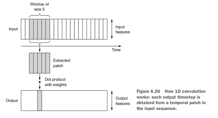
1D Convolution

1D convolution is used for sequential data. The input is a sequence \(I = (I(1), \ldots, I(T))\), and the convolution kernel \(K\) has \(k\) elements. The feature map is:

\[ S(i) = \sum_{t=-\frac{k-1}{2}}^{\frac{k-1}{2}} I(i+t)K(t) \]

1D convolution is commonly used in time series processing and text convolution in NLP.

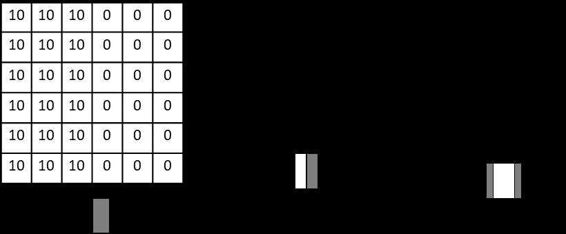
The following figure shows an example of edge detection using a convolution kernel — a vertical edge detection filter enables the convolution operation to automatically extract vertical edges from the image:

Output Size of 2D Convolution

For an input of size \(H \times W\) and a kernel of size \(k \times k\), without padding, the output size is:

\[ (H - k + 1, \quad W - k + 1) \]

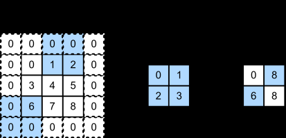
Padding

The purpose of padding is to control the spatial dimensions of the output, typically to maintain the same size as the input. In PyTorch:

• padding='valid': No padding, output size is \((H-k+1, W-k+1)\)
• padding='same': Zeros are padded around the input so the output has the same spatial dimensions as the input

Stride

Stride refers to the number of pixels the kernel moves at each step. The default stride is 1; a stride greater than 1 enables rapid downsampling of the input image:

• Higher computational efficiency
• Rapidly reduces feature map dimensions
• Particularly useful with larger kernels

With stride \(s\), the output size is reduced to approximately \(1/s\) of the original size.

---

Finally, we need to explain the concept of "channels".

Since input images are typically three-dimensional (e.g., an RGB image has red, green, and blue channels), the hidden layers within the network also use three-dimensional tensors. Each hidden representation consists of multiple 2D grids stacked together, known as "channels" or "feature maps."

Intuitively, lower-level channels near the input specialize in recognizing simple geometric features (such as edges), while higher-level channels recognize more complex patterns (such as textures or object parts).

To support multiple input and output channels, the weight \(\mathsf{V}\) introduces a fourth dimension:

\[ [\mathbf{H}]_{i,j,d} = \sum_{a=-\Delta}^{\Delta} \sum_{b=-\Delta}^{\Delta} \sum_{c} [\mathsf{V}]_{a,b,c,d} [\mathbf{X}]_{i+a, j+b, c} \]

• Index \(d\)* : Represents the *output channel. Each \(d\) corresponds to a unique convolution kernel responsible for generating one layer of the output tensor.
• Index \(c\)* : Represents the *input channel. The kernel convolves across all input channels and sums the results.
• Weight \(\mathsf{V}\)**** : Here it is a four-dimensional tensor, typically shaped as (kernel height, kernel width, input channels, output channels).

Convolution Kernel

For a grayscale image, we can use a 3x3 convolution kernel. In this case, we can think of a single convolution operation as stamping — one stamp covers 9 points, and we obtain a single number.

For an RGB image, since RGB images have 3 channels (red, green, blue), each convolution kernel must also have 3 layers to match these channels. This \(3 \times 3 \times 3\) kernel block slides across the image. It simultaneously examines the red, green, and blue layers, multiplying the 27 values (\(3 \times 3 \times 3\)) by the corresponding pixels and summing them all, ultimately producing a single value.

Note that a color image is essentially three images — the R, G, and B grids. Imagine these three images stacked together, and our stamp pressed into them like a thick cookie cutter covering 9 points on each of the RGB layers simultaneously. We multiply the weights corresponding to all 9x3=27 points and add them together, still obtaining just a single number.

In other words, regardless of how the kernel is designed, the goal is for each kernel to output a single number.

As we slide this kernel across the image, the numbers produced by the kernel are arranged into a flat feature map.

One kernel produces one feature map. In deep learning, we want a single convolutional layer to extract multiple features simultaneously. Therefore, we typically use multiple different kernels to obtain multiple different feature maps.

For example, if we use 64 kernels to learn to recognize different features, each of these 64 different kernels produces one feature map. Stacking these 64 feature maps together forms the hidden representation \(\mathbf{H}\)**** mentioned in previous sections, which has 64 channels.

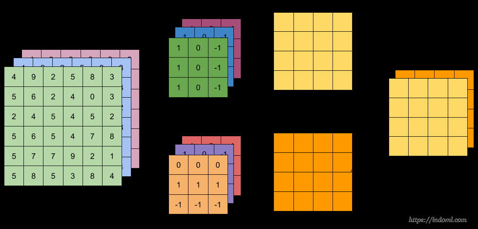
For multi-channel (\(C\) input channels) 2D convolution:

• Input size: \(H \times W \times C\)
• Single kernel size: \(k \times k \times C\)
• Without padding, output size: \(H' \times W' \times 1\), where \(H' = H - k + 1\), \(W' = W - k + 1\)
• With \(C'\) kernels, total kernel size: \(k \times k \times C \times C'\), output size: \(H' \times W' \times C'\)

---

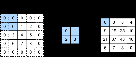
Temporarily ignoring the third dimension (channels), let us consider a 2D example. Below is the 2D cross-correlation operation: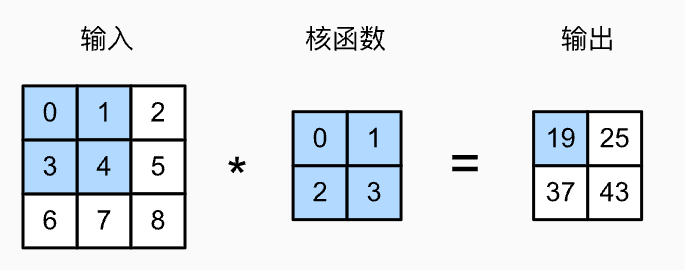

The computation involves element-wise multiplication between the region covered by the kernel and the corresponding kernel values, then summing the results: 0x0+1x1+3x2+3x4=19.

Convolutional Layer

We have already learned what a convolution kernel is. We also mentioned that recognizing and extracting multiple different features requires multiple kernels.

In neural networks, we place multiple kernels in a single layer to form a convolutional layer.

When building networks in practice, convolutional layers are typically configured according to three principles:

1. As depth increases, width increases. Layers closer to the input (lower layers) generally have fewer kernels, since the feature maps are still large at that point. Layers closer to the output generally have more kernels, where the spatial dimensions have been compressed, so the primary goal is to compose more complex abstract semantics.
2. Receptive Field: By stacking multiple \(3 \times 3\) convolutional layers, the network can see progressively larger image regions. Two stacked \(3 \times 3\) convolutions have the same field of view as a single \(5 \times 5\) convolution, but with fewer parameters and stronger nonlinear expressiveness.
3. Since we typically use GPUs for computation, setting the number of channels to a multiple of 8 enables faster GPU execution, as this better aligns with NVIDIA GPU memory alignment and Tensor Core computation logic.

Learnable Parameters

The number of learnable parameters in a convolutional layer is the total size of all kernels: \(k \times k \times C \times C'\) (excluding bias), where \(k\) is the kernel size, \(C\) is the number of input channels, and \(C'\) is the number of output channels. The total parameter count of a CNN is the sum of parameters across all convolutional and fully connected layers.

CNN Terminology

• Receptive Field: The region of the input image corresponding to a particular output unit. The receptive field grows larger as the network gets deeper
• Kernel/Filter: The convolution filter, also called the convolution kernel
• Feature Map: The hidden layer output after a convolutional or pooling layer
• Layer Counting: Typically refers to the number of transformation layers (convolutional and fully connected layers), excluding pooling layers and activation functions

Representation and Emergence

Representation is the process of transforming "raw data" into a "form that machines can easily understand" (features/vectors).

Representation

Let us use an intuitive example: recognizing a photo of a "cat".

Raw Data (Input):

• For a computer, this is just a matrix of numbers (e.g., \(224 \times 224 \times 3\) pixels).
• These numbers are very chaotic. Slightly shifting the cat's position or dimming the lighting changes all pixel values.
• At this level, the computer cannot distinguish between a "cat" and a "dog."

Good Representation:

• Suppose after passing through a CNN, the final layer transforms these pixels into a vector (e.g., a 128-dimensional array).
• Each number in this vector no longer represents pixel brightness, but rather "semantic features":
  • Dimension 1: Are there pointed ears? (1=yes, 0=no)
  • Dimension 2: Is it furry?
  • Dimension 3: Are there whiskers?
• This vector is the "representation" of the image.

Core Logic:

• Pixel space: Images of cats and dogs are mixed together, inseparable by a single line (linearly inseparable).
• Representation space: Cat vectors cluster together, dog vectors cluster together. Easy to separate (linearly separable). *

If you understand representation, you understand the paradigm-shifting advantage of deep learning over traditional machine learning.

Traditional Machine Learning (Old School)

• Approach: Hand-crafted features.
• Pain point: Want to recognize cats? You need to manually write algorithms to extract edges (Sobel), textures (Gabor), and keypoints (SIFT). These feature extractors are human-designed and rigid. If you switch to recognizing "birds," you need to redesign the entire pipeline.
• Bottleneck: Human intelligence limits the model's ceiling.

Deep Learning

• Approach: End-to-End Representation Learning.
• Revolutionary aspect: We no longer tell the model to "find edges" or "find textures." We only provide raw pixels and labels (cat/dog). The network discovers on its own the best way to represent the data (the hierarchical emergence in CNNs we discussed earlier).
• Advantage: Machine-learned representations are often more abstract, more robust, and more useful than human-designed ones.

Representation can be viewed as the output vectors of intermediate network layers. Common forms of representation include:

Embedding:

• In NLP, transforming a word ("Apple") into a vector. This vector is its representation.
• If the representation is well-learned, the vectors for "Apple" and "Orange" will be close, while "Apple" and "Car" will be far apart.

Latent Code:

• In VAEs or Autoencoders, the compressed vector \(z\) in the middle is the representation.
• It captures the "essence" of the data.

Feature Map:

• In CNNs, the output of each layer is a form of representation.
• Shallow representations: lines, colors.
• Deep representations: eyes, ears.

Representation Learning

In short, representation learning is the process of letting machines automatically discover the best way to describe data.

To enable a machine to recognize a "cat" in an image, there are two approaches:

• Traditional approach (manual feature engineering): Scientists tell the computer: "Cats have pointed ears, long whiskers, and round eyes." Programmers must write complex algorithms to define what "pointed" and "round" mean. This is manual representation design. The drawback is extreme rigidity — change the angle or lighting, and the program fails.
• Representation learning (deep learning): You do not tell the computer what a cat looks like; you simply show it tens of thousands of cat photos. Through hidden layer weight adjustments, the computer spontaneously discovers features such as "edges," "curves," and "fur textures." It learns on its own how to condense a complex pixel image into a set of efficient mathematical vectors.

Representation learning is essentially performing feature extraction and dimensionality reduction.

• Raw data (low-level representation): A mass of meaningless pixels (RGB values) — voluminous and chaotic.
• Learned data (high-level representation): A sequence of numbers from the higher layers of a neural network. These numbers may represent "there is a circle here" or "there is a contour here."

Although CNN's representation learning is the most visually apparent, all deep neural networks (DNNs) follow the same philosophy.

Before deep learning became popular, machine learning primarily relied on shallow models, characterized by very few layers (typically only 1-2 hidden layers, or even none).

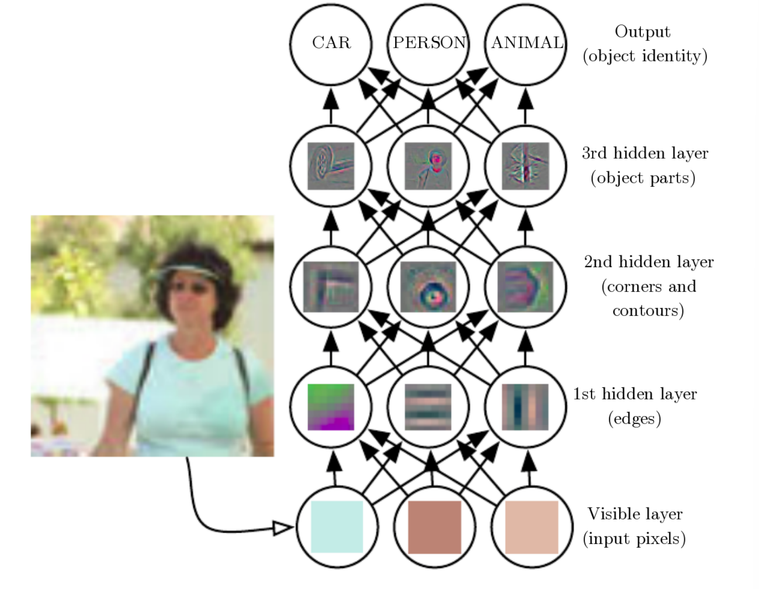
Although the Universal Approximation Theorem mathematically proves that a feedforward neural network with a single hidden layer and sufficiently many neurons can approximate any continuous function on a closed interval to arbitrary precision, in reality, the logic of nature is itself multi-layered and progressively abstract. As the renowned scholar Yoshua Bengio stated: "Deep architectures have a prior that better captures the complexity of the natural world." This prior is the hierarchical structure shown in the figure.

This is analogous to how we can replace all multiplication with addition, yet we still need multiplication. Different tools have vastly different effectiveness in practice.

Emergence of Internal Representations

In CNNs, we pre-design the growth rules: shallow kernels are small, and depth increases progressively. The CNN architecture itself does not prescribe discovery targets for different layers, yet the architecture we designed has been found a posteriori to exhibit compositionality. In other words, the CNN independently discovered certain universal laws of the physical world. If we visualize the features learned internally by a CNN, we find that shallow convolutions extract edges, lines, and textures, while deep convolutions identify eyes, wheels, complete birds, and so on.

Through exposure to massive amounts of images, the CNN learned capabilities akin to the biological visual nervous system — this is an emergence phenomenon. We only designed a layer-by-layer stacking structure, yet the CNN discovered a posteriori that layer-by-layer recognition minimizes the loss and that this is the only viable path — this was the first significant instance of compositional emergence in the history of neural network development, namely hierarchicalization.

• 1987 (NetTalk): Emergence of single concepts like "vowel/consonant."
• 2012 (AlexNet): Emergence of a complete evolutionary tree:
  • Layer 1: Physical layer (lines).
  • Layer 2: Geometric layer (circles, textures).
  • Layer 3: Part layer (eyes, wheels).
  • Layer 4: Semantic layer (cats, cars).

This continuous evolution from physical to semantic, was the first time humanity clearly observed the concretization of a "cognitive process" inside a machine.

Core Components of CNN

After years of development, from LeNet-5 to ResNet, the core components of modern CNNs have largely been established. We summarize them here.

Conv Layer

The Convolution Layer is the core computational unit and the foundation of CNN, responsible for local feature extraction.

The essential roles of a convolutional layer:

• Spatial feature extraction
• Weight sharing
• Local receptive field modeling

Activation

The introduction of ReLU dramatically improved the trainability of deep networks (as demonstrated in AlexNet).

Common forms:

• ReLU
• Leaky ReLU
• GELU
• SiLU / Swish

Batch Normalization

ResNet introduced BatchNorm and demonstrated its importance.

Common types:

• BatchNorm (BN)
• LayerNorm
• GroupNorm

Used for:

• Stabilizing training
• Accelerating convergence
• Mitigating gradient explosion/vanishing

Note: In CNNs, BN uses the same normalization parameters for an entire channel (i.e., each channel shares one set of \(\gamma\) and \(\beta\)) to preserve spatial continuity between image pixels. This differs from fully connected layers, where each feature dimension is normalized independently.

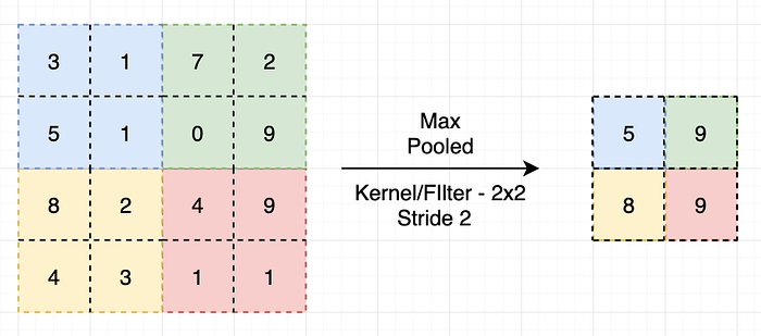
Downsampling

Used to expand the receptive field and reduce computation:

• MaxPooling
• AveragePooling
• Convolution with Stride > 1

Modern architectures increasingly prefer stride convolution over pooling.

Pooling layers aggregate detected patterns within local regions and have two parameters: pool size and pool stride, where pool size typically equals pool stride.

Skip Connection

The residual network proposed in ResNet fundamentally changed CNNs, proving that networks can be very deep.

Advantages:

• Improved gradient flow
• Enables construction of extremely deep networks (>100 layers)

Before ResNet, deep stacking structures without residual connections suffered from vanishing gradients and performance degradation — for example, 20+ layers of pure convolution + ReLU (without skip connections). After ResNet, such structures virtually disappeared.

Head

Modern CNNs rarely use large-scale fully connected layers, instead employing:

• Global Average Pooling (GAP)
• Fully connected layers (small-scale)
• Softmax / task output layers

Typical structure:

Feature Map
   ↓
Global Avg Pool
   ↓
Linear
   ↓
Softmax

.

Retired Components

Throughout the evolution of CNNs, some once-pioneering components have essentially been retired.

Sigmoid/Tanh

These two activation functions were the first to be retired, and the advent of ReLU marks the beginning of modern CNNs.

Large Fully Connected Layers

Representative architectures include AlexNet and VGGNet, characterized by:

• 4096 x 4096 scale FC layers
• Extremely high parameter proportion (>80%)
• Heavy reliance on Dropout to prevent overfitting

Why retired:

• Extremely low parameter efficiency
• Prone to overfitting
• Unfavorable for transfer learning

Modern replacement:

• Global Average Pooling (GAP)
• Lightweight linear layers

Dropout

Dropout is effective in:

• FC layers
• Small data scenarios

However, in modern CNNs:

• BatchNorm is available
• Data augmentation is used
• Residual structures exist
• Stronger regularization (e.g., weight decay) is employed

Dropout actually:

• Disrupts BN statistics
• Slows convergence

Therefore, it is often removed from CNN backbones and only remains common in:

• Small data settings
• Transformers
• Head layers

LRN

Local Response Normalization primarily appeared in:

• AlexNet

Purpose:

• Simulating neuronal inhibition
• Early training stabilization

Why retired:

• BatchNorm is more effective
• Faster convergence
• Clearer theoretical foundation

Now almost entirely replaced by BatchNorm / GroupNorm.

Pooling-Dominant Downsampling

Examples:

• VGG-style extensive MaxPooling
• Fixed-position downsampling

Problems:

• Irreversible information loss
• Not learnable

Modern trends:

• Strided convolution replaces pooling
• Sometimes pooling is removed entirely

CNN Visualization

CNN visualization techniques help us understand the internal workings of the network. The analysis is conducted primarily along the following dimensions:

• Data dimension: selected training data vs. network-generated feature maps
• Analysis granularity: entire class activations vs. single filter stimuli
• Technical methods: backpropagation to input, deconvolution, occlusion, class activation mapping (CAM)

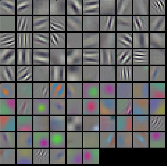
Visualizing Learned Filters

Directly visualizing the weights of first-layer convolution kernels. Image patches that share the same pattern as a filter are most likely to produce the highest response for that filter. This method is only applicable to the first layer, since deeper filters correspond to higher-dimensional input spaces that are difficult to visualize directly.

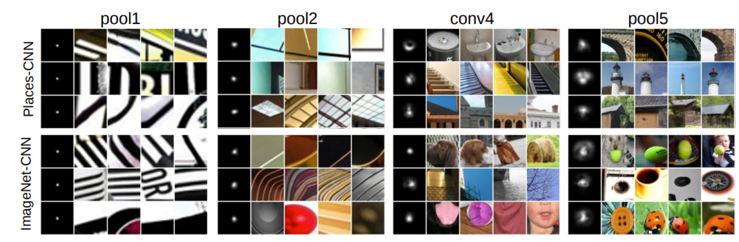
Filter Response

Finding image patches within the receptive field that produce the highest response for a given filter. These patches reveal the patterns that the filter attends to. As layers deepen, the patterns captured by filters evolve from simple edges and lines to complex object parts and semantic concepts.

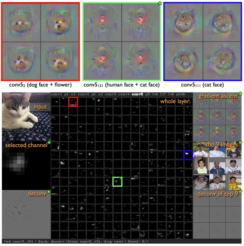
Other methods for analyzing filters include:

• Gradient Ascent Analysis: Starting from a blank image, optimizing to find the image that maximizes a particular filter's response
• Deconvolution Analysis (Deconv): The filter extracts relevant information from the image and removes irrelevant "noise"; the deconvolution operation attempts to recover the input from the extracted information, and the recoverable portion indicates the filter's focus
• Saliency Maps: High-response regions in a channel indicate the filter's areas of attention

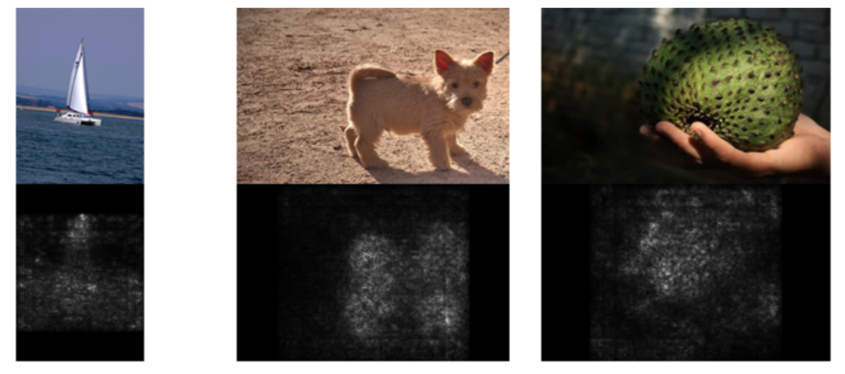
Gradient Visualization and Saliency Maps

Saliency maps indicate the regions that a CNN focuses on. By computing the gradient of the output with respect to the input image, regions with large gradient values (regardless of sign) represent the CNN's areas of attention, while the CNN exhibits low gradient values for irrelevant pixels (such as background regions).

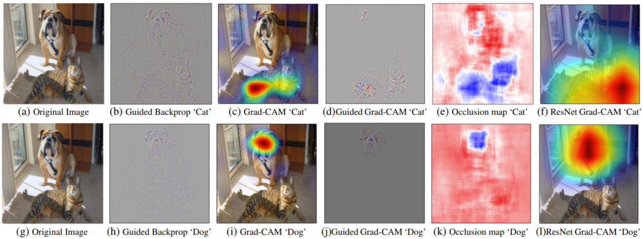
Class Activation Mapping (CAM / Grad-CAM)

CAM (Class Activation Map) highlights the image regions that contribute most to a particular class score. Grad-CAM generalizes this method to a wider range of network architectures through gradient weighting, generating class-discriminative heatmaps without requiring network modification. Occlusion saliency maps locate key regions by occluding different areas of the input image and observing the change in output.

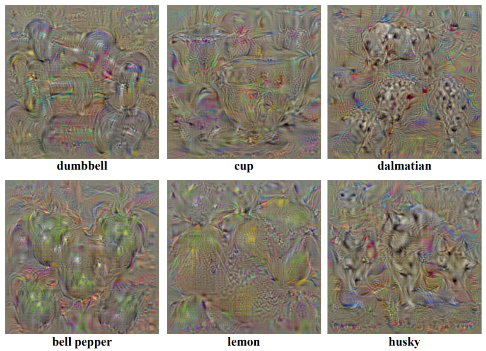
Gradient Ascent for Generating Class-Typical Images

By maximizing the score of a particular class, gradient ascent optimization is performed on a blank image to generate a "typical image" of that class. The generated images reveal the visual features that the network considers characteristic of that class.

---

评论