Image Segmentation
Pixel-Level Tasks
Unlike image classification, which assigns a single label to an entire image, pixel-level tasks require making a prediction for every individual pixel. Equivalently, this amounts to partitioning an image into distinct regions where all pixels within each region belong to the same category.
Common pixel-level tasks include:
- Semantic Segmentation: Partitioning an image into multiple regions, each corresponding to a particular "object" class
- Instance Segmentation: Building on semantic segmentation by further distinguishing between different instances of the same class
- Medical Applications: Detecting tumors in X-rays or delineating cell boundaries in microscopy images
- Image Generation: A network takes a noisy image as input and predicts a cleaner version of it
Principles
Nearly all segmentation CNNs follow an Encoder + Decoder architecture:
输入图像
   ↓
Encoder (CNN提取特征)
   ↓
Decoder (上采样恢复尺寸)
   ↓
像素分类图
The decoder typically relies on:
- Transposed Convolution
- Upsampling
Transposed Convolution
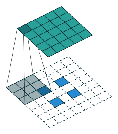
Transposed convolution maps a small-sized input to a larger-sized output, serving as the spatial "inverse" of a standard convolution:
- Mechanism: If a standard convolution with stride \(s\) spatially shrinks an image, a transposed convolution with stride \(s\) spatially enlarges it
- Internal padding: Expansion is achieved by inserting zeros between input pixels and then applying a convolution kernel
- "Inverse" shape: By design, it is the spatial inverse of convolution — if a \(4 \times 4\) input is reduced to \(2 \times 2\) by a convolution, a transposed convolution can restore the \(2 \times 2\) back to \(4 \times 4\)
Transposed convolution is also referred to as "deconvolution" or "up-convolution," though the term "deconvolution" is technically a misnomer since the operation is not the mathematical inverse of convolution.
U-Net
U-Net is one of the most influential architectures in image segmentation. Its symmetric encoder–decoder structure and skip connection design have inspired a vast body of subsequent work.
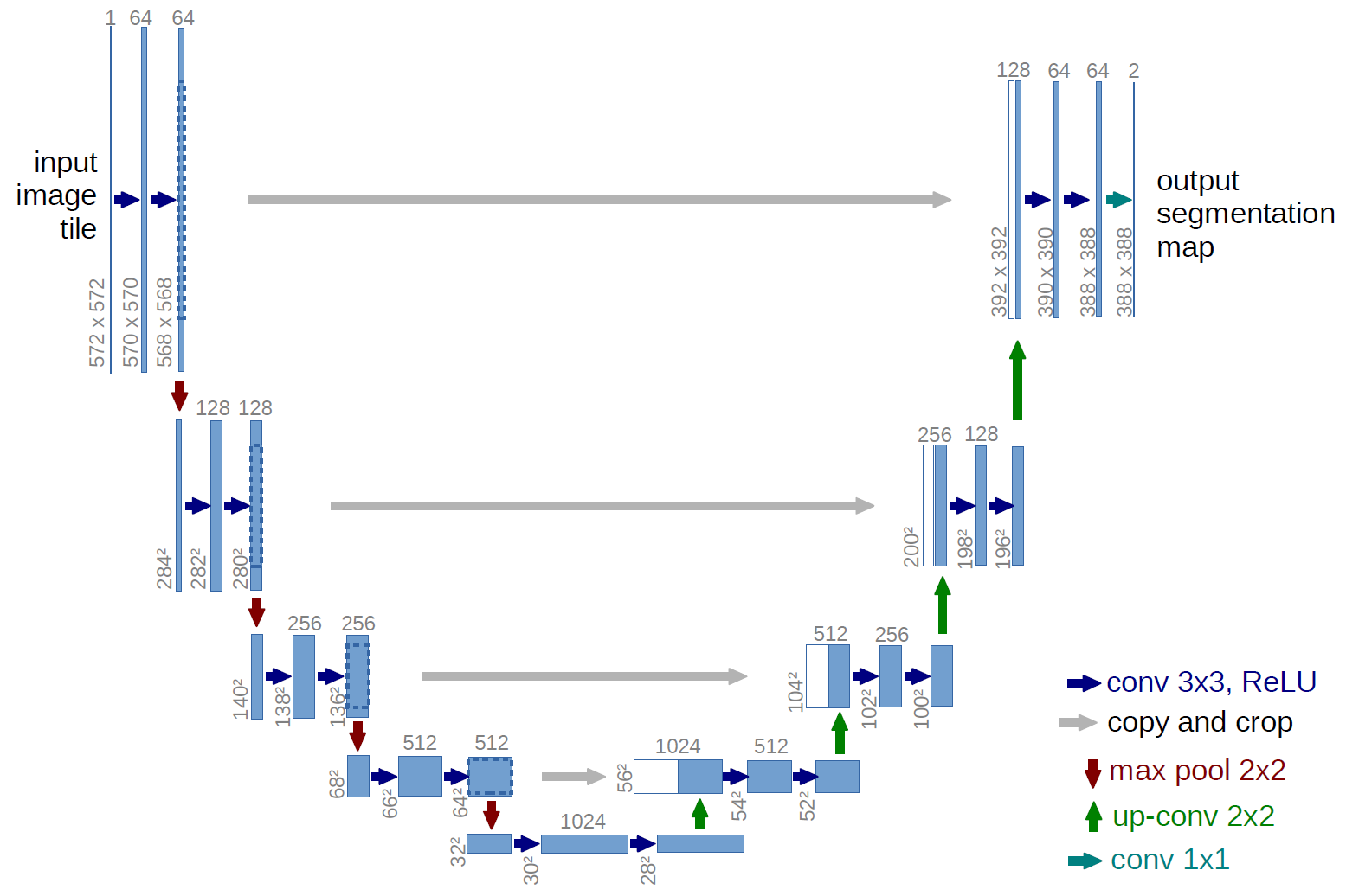
Architecture
U-Net has a symmetric architecture composed of two paths:
Contracting Path (Encoder):
- Follows the architecture of a typical convolutional network
- Repeatedly applies two \(3 \times 3\) convolutions (each followed by ReLU), then a \(2 \times 2\) max pooling operation for downsampling
- The number of feature channels is doubled at each downsampling step
Expansive Path (Decoder):
- Each step upsamples the feature map, followed by a \(2 \times 2\) transposed convolution ("up-convolution")
- Skip Connections: This is U-Net's "secret weapon" — feature maps from the corresponding layer in the contracting path are concatenated with the upsampled feature maps. This allows the network to leverage high-resolution, fine-grained features from earlier layers for precise localization
- A final \(1 \times 1\) convolution maps each feature vector to the desired number of classes
FCN (Fully Convolutional Networks)
FCN (Long et al., 2015) is the foundational work in semantic segmentation, demonstrating for the first time that end-to-end pixel-level prediction is feasible.
Core Idea
FCN replaces the fully connected layers in traditional classification networks (e.g., VGG-16) with convolutional layers, enabling the network to accept inputs of arbitrary size and produce correspondingly sized segmentation maps.
Key modifications:
- Replace the three fully connected layers (fc6, fc7, fc8) in VGG-16 with \(1 \times 1\) convolutional layers
- The final output has \(C\) channels (one per class), each representing a probability map for that class
- Use transposed convolutions to upsample the low-resolution feature map back to the original input size
Skip Connections
Directly upsampling the last feature map produces overly coarse outputs. FCN introduced skip connections to fuse features from different levels:
- FCN-32s: Directly upsample the last layer (pool5) by 32x — coarse results
- FCN-16s: Fuse pool5 (upsampled 2x) with pool4 features, then upsample 16x
- FCN-8s: Further fuse pool3 features, upsample 8x — richer details
Skip connections allow the network to leverage both high-level semantic information ("what is it") and low-level spatial information ("where is it"), significantly improving the fineness of segmentation boundaries.
DeepLab Series
The DeepLab series (Google Research) is among the most influential work in semantic segmentation, evolving from v1 through v3+.
Atrous Convolution (Dilated Convolution)
Standard convolution expands the receptive field slowly, while pooling layers enlarge it at the cost of spatial resolution. Atrous convolution expands the receptive field by inserting zeros (holes) between kernel elements while keeping the feature map resolution unchanged.
For an atrous convolution with dilation rate \(r\), the effective receptive field size is:
where \(k\) is the original kernel size. For example, a \(3 \times 3\) kernel with \(r=2\) has an effective receptive field of \(5 \times 5\), and with \(r=3\) it becomes \(7 \times 7\).
ASPP (Atrous Spatial Pyramid Pooling)
The ASPP module applies multiple atrous convolutions with different dilation rates in parallel to capture multi-scale contextual information:
- Uses multiple branches with rates such as \(r = 6, 12, 18, 24\) (exact values vary by version)
- Each branch captures context at a different scale
- Branch outputs are concatenated or summed for fusion
- DeepLabv3 additionally includes a global average pooling branch to capture image-level features
CRF Post-Processing
DeepLabv1 and v2 employ a Dense Conditional Random Field (Dense CRF) as a post-processing step to refine segmentation boundaries:
- CNN-produced segmentation maps typically have blurry boundaries
- CRF leverages spatial relationships and color similarity between pixels to sharpen boundaries
- The energy function consists of unary potentials (CNN predictions) and pairwise potentials (inter-pixel relationships)
DeepLabv3+
DeepLabv3+ (2018) combines the encoder-decoder architecture with ASPP:
- Encoder: Uses a modified Xception or ResNet as the backbone, combined with the ASPP module
- Decoder: Upsamples the encoder output by 4x, concatenates it with corresponding low-level features from the backbone, refines through convolutions, and upsamples by another 4x to restore the original resolution
- Depthwise separable convolution: Widely used in both the ASPP and decoder to reduce computational cost
Mask R-CNN
Mask R-CNN (He et al., 2017) extends Faster R-CNN by adding a segmentation branch, achieving instance segmentation.
Architecture
Mask R-CNN adds a mask prediction branch in parallel to Faster R-CNN's detection framework:
- Classification branch: Predicts the object class
- Regression branch: Predicts the bounding box
- Mask branch: Predicts an \(m \times m\) binary mask for each RoI
All three branches share the same feature extraction backbone (e.g., ResNet-FPN). Classification and regression determine "what" and "where," while the mask branch determines "the precise shape."
RoI Align
The key innovation in Mask R-CNN is replacing RoI Pooling with RoI Align:
- Problem with RoI Pooling: Both the RoI boundaries and pooling grid require quantization (rounding), and this quantization error is especially severe for small objects
- RoI Align's improvement: Uses bilinear interpolation to precisely compute feature values at each sampling point, avoiding any quantization
RoI Align eliminates spatial quantization errors and yields particularly significant improvements in mask prediction quality.
Loss Function
The total loss in Mask R-CNN is the sum of three components:
where \(L_{\text{mask}}\) is a per-pixel binary cross-entropy loss computed independently for each class on each RoI. This class-decoupled design prevents competition between different classes.
Panoptic Segmentation
Panoptic segmentation (Kirillov et al., 2019) unifies semantic segmentation and instance segmentation.
Definition
- Semantic segmentation: Assigns a class label to every pixel without distinguishing between different instances of the same class
- Instance segmentation: Identifies and segments each individual object instance but does not handle background regions
- Panoptic segmentation: Combines both — assigns semantic labels to all pixels while also distinguishing different instances of "thing" categories (countable objects such as people and cars)
Category Taxonomy
- Things (countable objects): People, cars, animals — objects with clear boundaries that require instance-level segmentation
- Stuff (uncountable regions): Sky, road, grass — background regions that only require semantic-level segmentation
Panoptic Quality (PQ)
The PQ evaluation metric for panoptic segmentation jointly measures recognition quality and segmentation quality:
SAM (Segment Anything Model)
SAM (Kirillov et al., 2023, Meta AI) is a general-purpose segmentation foundation model designed to handle segmentation tasks across arbitrary scenarios.
Core Design
SAM consists of three components:
- Image Encoder: Uses a pretrained ViT (Vision Transformer) to extract image features; needs to run only once per image
- Prompt Encoder: Encodes various types of user prompts
- Mask Decoder: A lightweight Transformer decoder that generates segmentation masks based on image features and prompt features
Prompt-Based Segmentation
SAM supports multiple types of prompts to specify the segmentation target:
- Point prompts: Foreground or background points
- Box prompts: Bounding boxes
- Text prompts: Natural language descriptions (supported in later versions)
- Mask prompts: Coarse input masks
This design gives SAM powerful zero-shot generalization — it can perform segmentation without any task-specific fine-tuning.
SA-1B Dataset
SAM was trained on over 11M images with 1.1B mask annotations, the largest segmentation dataset to date. The annotation process used a model-assisted interactive labeling pipeline, dramatically improving labeling efficiency.
Significance
SAM marks the entry of the segmentation field into the "foundation model" era:
- Generality: A single model handles a wide range of segmentation tasks
- Interactivity: Prompts flexibly specify segmentation targets
- Zero-shot transfer: Applicable to new domains without fine-tuning
Evaluation Metrics
IoU (Intersection over Union)
IoU is the most fundamental evaluation metric for segmentation tasks, measuring the overlap between predicted and ground-truth regions:
where \(P\) is the predicted segmentation region and \(G\) is the ground-truth annotation region.
mIoU (mean IoU)
mIoU is the average IoU across all classes and serves as the most commonly used comprehensive metric for semantic segmentation:
where \(C\) is the total number of classes. mIoU assigns equal weight to each class, preventing large classes from dominating the evaluation.
Dice Coefficient
The Dice coefficient (also known as the pixel-level F1 Score) is particularly common in medical image segmentation:
The relationship between Dice and IoU is:
The Dice coefficient is always greater than or equal to IoU. In practice, Dice Loss is frequently used as a training loss for segmentation networks:
where \(p_i\) is the predicted probability, \(g_i\) is the ground-truth label, and \(\epsilon\) is a smoothing term to prevent division by zero.