Machine Learning Fundamentals

This chapter covers the most essential concepts in machine learning, all of which are equally critical for deep learning. The content is primarily drawn from Chapter 5 of the IAN textbook.

What Is Machine Learning

In simple terms, machine learning refers to software systems that improve their capabilities by learning from data:

• Use examples data to teach (fit) a model.
• Use the model to make decisions.

Traditional tasks such as spam detection and face recognition are easy to describe but difficult to define (what exactly counts as spam) or to program explicitly (face recognition).

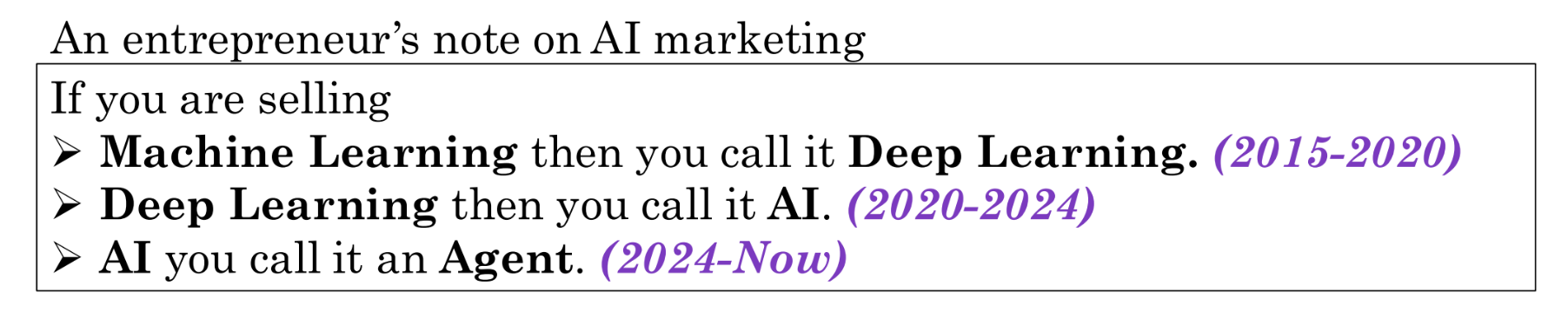
Today, machine learning is often used interchangeably with artificial intelligence, because the core tools and techniques behind modern AI are rooted in machine learning. Put another way: our ultimate goal remains artificial intelligence; machine learning is simply the most effective tool we have right now. The ultimate aim of AI is to endow computing systems with human-like intelligence capable of learning, reasoning, problem-solving, perception, decision-making, and more.

In general, machine learning falls into the following categories:

(1) Supervised Learning:

• Classification: predict a categorical output Y from input X

  • Image recognition: predict a label from an image
  • ChatGPT: predict the next word given a prompt
  • Regression: predict future continuous values Y from historical data X
  • Stock price prediction
  • Image, Video Generation

(2) Unsupervised Learning:

• Clustering & Density Estimation
• Dimensionality Reduction

(3) Reinforcement Learning

Reinforcement learning is typically studied as a separate topic. Our course focuses primarily on supervised and unsupervised learning.

---

Historical timeline of ML:

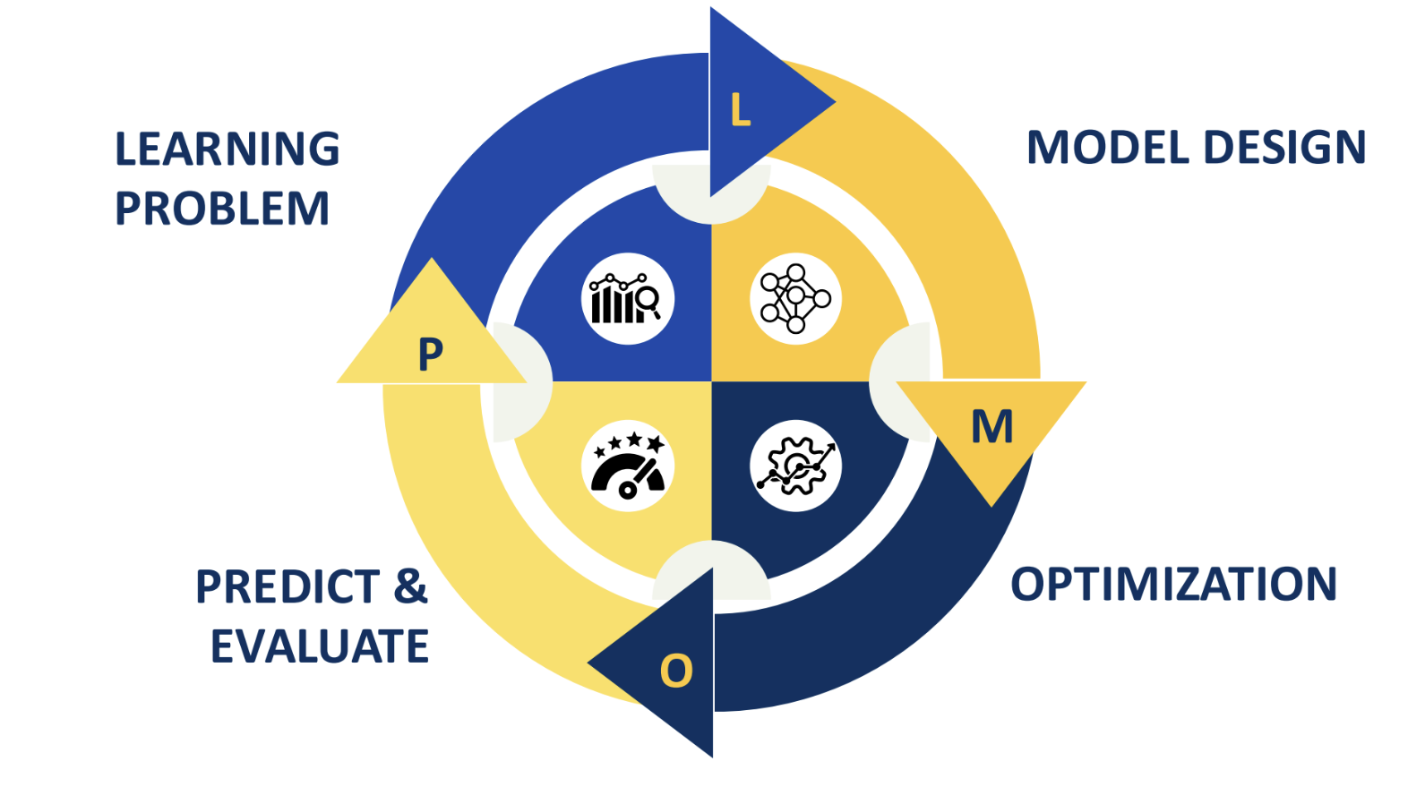
ML Lifecycle:

---

Formal Definition

The most authoritative definition of machine learning was given by Tom Mitchell:

A computer program is said to "learn" from experience \(E\) with respect to some task \(T\) and performance measure \(P\), if its performance on \(T\), as measured by \(P\), improves with experience \(E\).

To constitute a "machine learning" process, the following three elements are indispensable:

• Task \(T\) (Task): The type of problem the system aims to solve.
  • Examples: classification (determining whether an email is spam), regression (predicting house prices), generation (writing a piece of copy).
• Experience \(E\) (Experience): Typically refers to data. The system discovers patterns by processing this data.
  • Form: Feature vectors \(x\) (e.g., pixel values of an image, a person's height and weight).
• Performance Measure \(P\) (Performance Measure): The yardstick for how "smart" the model is.
  • Examples: error rate, accuracy, value of the loss function.

At its core, the "learning" in the definition of machine learning is really about finding a target function \(f\). Mathematically, we assume there exists a perfect function in the real world (e.g., \(f(\text{image}) = \text{cat}\)), but this function is too complex for humans to write out. Machine learning uses experience \(E\) to iteratively reduce the error, ultimately producing an approximate function \(\hat{f}\) that performs as closely to \(f\) as possible under the performance measure \(P\).

Common machine learning tasks include:

• Classification: \(E\) is a labeled dataset (e.g., photos with cat/dog labels); \(P\) is accuracy, precision, recall, F1 score, etc.
• Regression: \(E\) is a dataset with numerical values (e.g., house features and sale prices); \(P\) is MSE, MAE, \(R^2\), etc.
• Clustering: \(E\) is an unlabeled dataset (e.g., large volumes of consumer spending records); \(P\) is silhouette coefficient, silhouette distance, etc.
• Reinforcement learning: \(E\) is feedback obtained through interaction with the environment; \(P\) is the cumulative reward.

---

To put it simply, machine learning is about finding the optimal set of model parameters that minimize prediction error on the known dataset:

\[ \boldsymbol{\theta}^* = \arg \min_{\boldsymbol{\theta}} \frac{1}{|D|} \sum_{(\boldsymbol{x}, y) \in D} L(y, f_{\boldsymbol{\theta}}(\boldsymbol{x})) \]

Where:

• \(f_{\boldsymbol{\theta}}(\boldsymbol{x})\) (prediction model): This is your model. It takes input data \(\boldsymbol{x}\) and, given the current parameters \(\boldsymbol{\theta}\) (e.g., neural network weights), produces a prediction.
• \(L(y, f_{\boldsymbol{\theta}}(\boldsymbol{x}))\) (loss function): This is the "scorecard." It measures the gap between the model's prediction \(f_{\boldsymbol{\theta}}(\boldsymbol{x})\) and the true label \(y\). The larger the gap, the higher the loss \(L\).
• \(\frac{1}{|D|} \sum_{(\boldsymbol{x}, y) \in D}\) (average loss): This part averages over the entire dataset \(D\). It sums the loss for every sample in the dataset and divides by the total number of samples \(|D|\), representing the average error rate across the entire training set.
• \(\arg \min_{\boldsymbol{\theta}}\) (finding the optimal parameters): The instruction: find the set of parameters \(\boldsymbol{\theta}\) that minimizes the average loss that follows.
• \(\boldsymbol{\theta}^*\) (optimal solution): The "perfect" parameters obtained after training.

Nearly all supervised learning algorithms — from simple linear regression to deep neural networks and even large language models like ChatGPT — execute this formula during training. However, not all machine learning models involve tuning parameters; there are also non-parametric models such as KNN or kernel-based SVMs.

After training on data, we need to assess whether the machine learning model works through generalization. Mathematically, this means computing the expected value of the loss function under the given data distribution:

\[ R(f) = \int_{(\boldsymbol{x}, y)} p(\boldsymbol{x}, y) L(y, f(\boldsymbol{x})) \text{d}(\boldsymbol{x}, y) \]

This generalization is fundamentally grounded in mathematical statistics, which is why this kind of generalization ability is also called statistical generalization. The symbols in the formula are interpreted as follows:

• \(R(f)\) (expected risk): The average loss of model \(f\) across all possible data. Note there is no \(\theta\) subscript here, because this is a universal definition applicable to any function \(f\).
• \(p(\boldsymbol{x}, y)\) (joint probability distribution): This is the most critical part. It represents the "ground truth" of the real world — the probability that a particular pair of input \(\boldsymbol{x}\) and label \(y\) co-occurs. In practice, we can never fully know this distribution.
• \(L(y, f(\boldsymbol{x}))\) (loss function): Same as before — the cost of making an incorrect prediction.
• \(\int_{(\boldsymbol{x}, y)} \dots \text{d}(\boldsymbol{x}, y)\) (integral): The mathematical "summation." It sweeps over all possible combinations of \(\boldsymbol{x}\) and \(y\) in the space, computing a weighted average according to their probabilities.

---

Since machine learning is fundamentally statistical in nature, different ML models inherently encode different inductive biases toward specific data patterns. In the context of machine learning, an inductive bias can be thought of as the model's prior hypothesis — an assumption it holds before seeing any data.

In other words, before the model ever encounters data, it already has an assumption about what the underlying pattern looks like. For example, linear regression assumes that if all data points are plotted on a coordinate system, there exists a line that can separate them. When multiple patterns can explain the current data, the model, based on its construction, favors one particular pattern over others.

As an illustration, imagine teaching two models to recognize fruit: one model assumes a linear hypothesis and believes fruits are round; the other assumes a color hypothesis and believes fruits are red. When they see a round, red apple, both can recognize it. But when shown a round, green watermelon, the linear-hypothesis model succeeds while the color-hypothesis model fails.

This inherent nature can be seen as either the model's innate talent or its built-in tinted glasses. In practice, one must choose different models based on the specific situation at hand.

The Essence of Function Approximation

No matter how complex a machine learning task appears, its central idea can always be understood as searching for an unknown target function that maps your input data to desired output results. In other words, the essence of machine learning is function approximation.

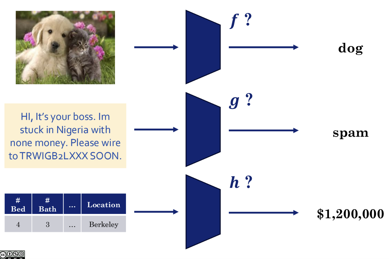
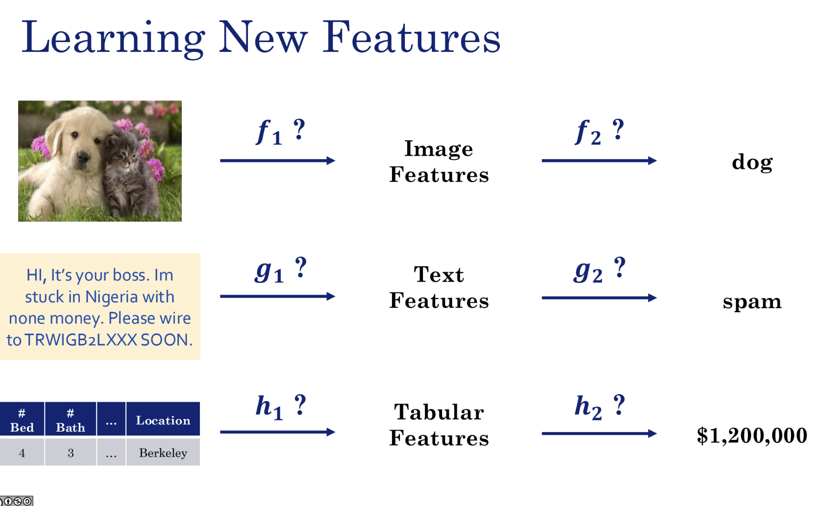
As shown in the figure above, whether the task involves image recognition, text recognition, or tabular data, the function capable of recognizing it is the machine learning model.

To enable computers to process real-world data, we must first convert various types of data into a unified, machine-readable format — numerical vectors.

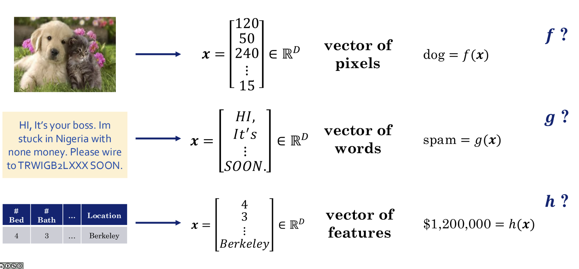
In the examples shown above:

• An image is converted into a long vector x composed of pixel values.
• Text is converted into a vector x composed of words.
• A table is converted into a vector x composed of individual features.

The machine learning model we seek is thus a function approximation capable of processing such data. That is, a machine learning model is essentially learning a function:

• Find a function f such that f(image vector) = "dog".
• Find a function g such that g(text vector) = "spam".
• Find a function h such that h(house feature vector) = "$1200000".

The process of model training is essentially the continuous adjustment of the model's internal parameters so that it approximates the ideal but unknown target function (i.e., the f, g, h mentioned above) as closely as possible.

In general, for a classic supervised learning model, two functions are of paramount importance:

1. Prediction Function: This is the f(x), g(x), h(x) mentioned above. This function is what we commonly refer to as the model itself — it receives input data x and produces a prediction y. It typically contains many tunable parameters, such as weights w and biases b. We use θ (theta) to denote the collection of all these parameters, so the prediction function is generally written as f(x; θ).
2. Loss Function (Cost Function): This is a function used to evaluate how well the model performs. It compares the gap between the model's prediction f(x; θ) and the true label y. The larger the gap, the higher the loss function value, indicating a worse model; the smaller the gap, the lower the loss, indicating a better model.

In other words, the essence of the training process is: continuously adjusting the parameters θ in the prediction function f(x; θ) to minimize the loss function L(θ). This process of finding the minimum is called optimization.

In summary, the essence of machine learning is defining an appropriate objective function for the problem. In the vast majority of supervised learning scenarios, the chosen objective function is the loss function, and our task is to find a set of model parameters that minimizes it. As noted earlier, reinforcement learning — one of the three major branches of machine learning — uses a reward function as its objective and seeks to maximize it.

To accomplish the above goals, we need to master the following mathematical tools:

• Linear algebra: for handling vectors and data
• Multivariate calculus: for optimizing the model and finding optimal parameters
• Probability theory: for handling uncertainty

For content related to mathematical tools, see the math notes.

---

Linear Algebra Perspective

Vectors

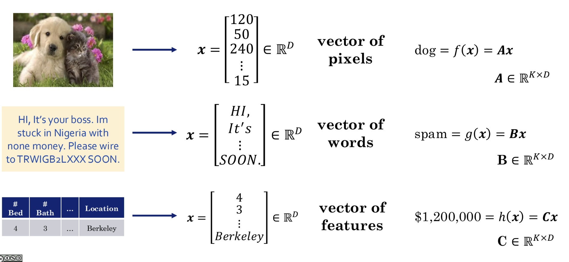
When we directly face a problem such as image recognition, it seems impossible to find a function f from scratch. So why not start with the simplest kind of function: a linear function. A linear function acting on vectors can be expressed as matrix multiplication:

• dog = f(x) = Ax
• spam = g(x) = Bx
• $1200000 = h(x) = Cx

In this way, an abstract problem is concretized and simplified into the problem of finding a specific matrix A. This is the key step from a machine learning concept to a linear algebra model.

So how do we analyze the function f(x) = Ax? Let us first review some general properties of functions in mathematics:

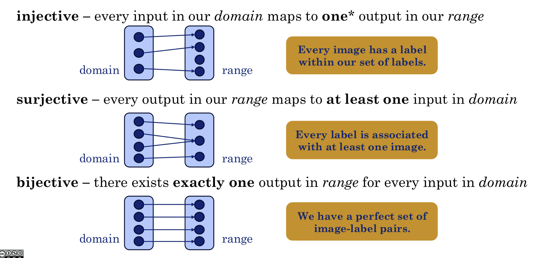
• Injective: each input maps to a unique output
• Surjective: every possible output has at least one corresponding input
• Bijective: inputs and outputs are in perfect one-to-one correspondence

Note that if a single input maps to multiple outputs, then it is not a valid function.

---

Dimensions

For classification and regression tasks, we can think of these as dimensionality reduction tasks, because the input information is always vast, complex, and high-dimensional, while the output is simple. Taking image recognition as an example, we want each image — regardless of how many there are — to map to one of a finite set of outcomes, so the ideal result is clearly a surjective mapping.

Of course, if our task involves dimensionality expansion — for instance, inputting a sentence (prompt) and generating an image — then it clearly cannot be surjective. From the task's perspective, a single input acts as a random seed whose result always corresponds to a unique image, making this clearly an injective mapping.

There is also the bijective case: for example, if we input a 100×100 image and output a 100×100 image, and the mapping is invertible, then it satisfies bijectivity.

Here, we call the input dimensionality D and the output dimensionality K:

• Dimensionality reduction: D > K, surjective mapping
• Dimensionality expansion: K > D, injective mapping
• Same dimensionality: D = K, bijective mapping

For the matrix function f(x) = Ax, A is a fixed transformation rule, x is our input vector, and f(x) = y is our output vector. When different x values are fed in, we obtain different y values. All such y values form a set called the range or column space. The dimension of this set is called the rank.

For example:

\[ A = \begin{bmatrix} 1 & 2 & 3 \\ 0 & 1 & 2 \\ 2 & 4 & 6 \end{bmatrix} \]

In this matrix, the third row is twice the first row, so the matrix contains redundant information. Therefore, the effective dimensionality of this matrix is only 2, i.e., rank(A) = 2, while the number of columns is 3, i.e., D = 3. We can use Gaussian Elimination to compute the rank of a matrix.

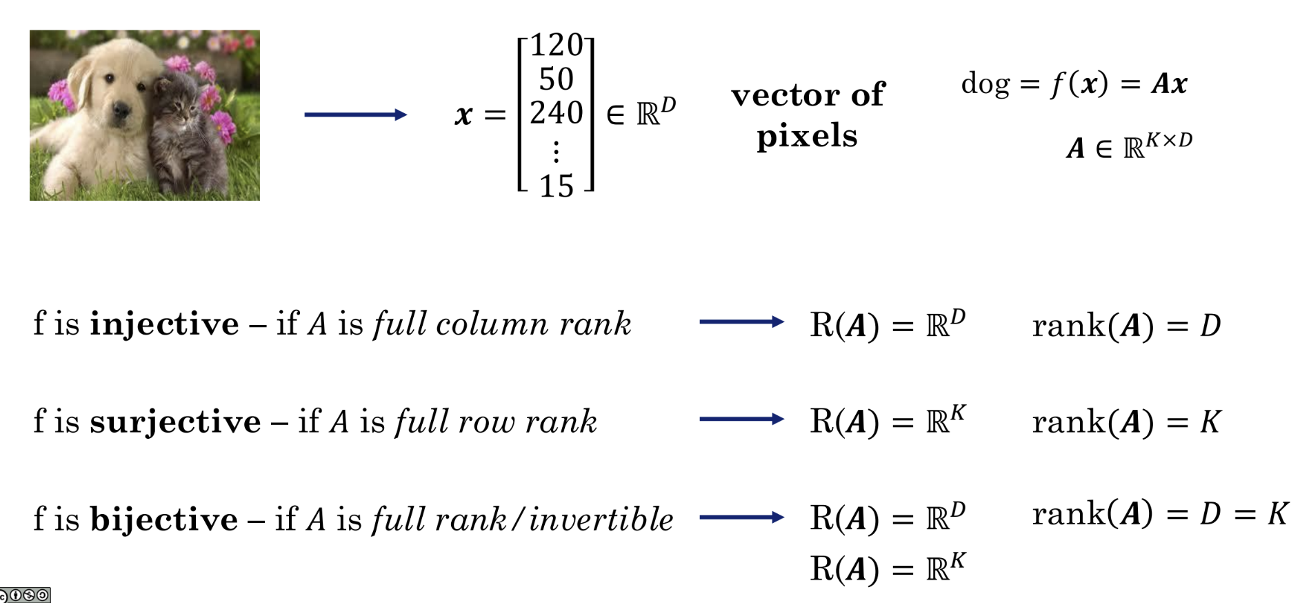
The figure illustrates the following properties from linear algebra:

f	A	rank(A)
f is injective	A is full column rank	rank(A) = D
f is surjective	A is full row rank	rank(A) = K
f is bijective	A is full rank/invertible	rank(A) = D = K

---

Iris Example

So how do we apply the knowledge above? Consider the classic iris classification problem: there are three species of iris (Setosa, Versicolor, Virginica). We measure four features for each flower: sepal length, sepal width, petal length, and petal width. The goal is to build a model that, given these four measurements, automatically determines which species the flower belongs to.

Before writing any code or choosing a model, let us first define conceptually what we are doing.

• We are looking for a function, which we name f.
• The input x to this function f should be a vector of 4 numbers (the 4 flower measurements). So x lives in a 4-dimensional space ℝ⁴ (D=4).
• The output y of this function f should tell us which of the 3 species it belongs to. A common approach is to let the output be a 3-dimensional vector, where each position represents the probability of belonging to a given species. For example, [0.9, 0.1, 0.0] might mean a 90% probability of being Setosa. So y lives in a 3-dimensional space ℝ³ (K=3).

Our abstract goal: find a perfect function f such that f(4 flower measurements) = probabilities for 3 species.

Next, finding an arbitrary, perfect f is too difficult. We decide to simplify by assuming that the unknown f can be well approximated by a linear function.

• Our concrete model: f(x) = Ax
• What is A?: A is the matrix that implements this linear function.
• Since the input x is 4-dimensional (D=4) and the output y is 3-dimensional (K=3), A must be a 3 x 4 matrix.
• A before training: Before we start training, A is just a 3x4 matrix filled with 12 random numbers. It knows nothing — it is a complete blank slate.

\[ A_{untrained} = \begin{bmatrix} ? & ? & ? & ? \\ ? & ? & ? & ? \\ ? & ? & ? & ? \end{bmatrix} \]

The new goal: Our task has been transformed from "finding an abstract f" to "finding the 12 best numbers for matrix A."

This process of finding the best A is also the core step of machine learning:

1. Prepare data: We gather a large collection of iris data, each with known 4 measurements (x) and the corresponding correct species (y_true).
2. Begin the loop:
   1. Take one flower's data x from the dataset.
   2. Feed it to our current matrix A and perform one matrix multiplication to get a prediction: y_pred = Ax.
   3. Compare our prediction y_pred with the true answer y_true to see how large the gap is. This "gap" is computed by the loss function.
   4. Use an optimizer (e.g., gradient descent) to slightly adjust the 12 numbers in matrix A based on this gap, updating A's parameters in the direction that reduces the loss.
3. Repeat: We repeat the above process for thousands of flowers in the dataset. The 12 numbers in matrix A are iteratively refined, little by little, until the loss becomes sufficiently small.

After training, A is no longer random numbers. It has become an "expert" containing patterns learned from the data.

\[ A_{trained} = \begin{bmatrix} -0.5 & 1.2 & -2.1 & -1.0 \\ 0.1 & 0.3 & 0.5 & -0.2 \\ 1.1 & -0.8 & 1.9 & 2.2 \end{bmatrix} \quad (\text{these numbers are illustrative}) \]

Now, the first row of matrix A, [-0.5, 1.2, -2.1, -1.0], is a learned "Setosa scorer" recipe. It has learned, for example, that the longer the petal length (the third feature), the less likely it is to be Setosa (because the coefficient -2.1 is negative).

At this point, training is complete. We can use our trained matrix to predict which class a new, unknown iris belongs to:

1. Measure: We measure its 4 features to get a new vector x_new.
2. Compute: We perform a simple matrix multiplication: y_new = A_trained * x_new.
3. Get the result: We obtain a 3-dimensional output vector, e.g., y_new = [0.85, 0.10, 0.05].
4. Interpret: This result tells us that the new flower has an 85% chance of being the Setosa species. We have successfully completed the prediction task.

To summarize:

• f: Our abstract conception of "an intelligent system that can recognize irises."
• A: The concrete tool (a 3x4 matrix) we chose to realize this conception.
• Training: The process of repeatedly refining and calibrating this tool through data (finding the best 12 numbers in A).
• Prediction: The process of using the refined tool (performing multiplication with the trained A) to solve new problems.

---

Calculus Perspective

Sensitivity of Functions

Multivariate calculus is also an important tool in machine learning. Let us return to the earlier discussion of ML as function approximation.

For a machine learning model y = f(x), how do we optimize or train this function? To answer this question, we must first understand the behavior of the function.

Imagine that our function f(x) is a house price prediction model:

• Input x is a vector of various house features, e.g., x₁ = area (square meters), x₂ = number of bedrooms, x₃ = distance to city center...
• Output y is the predicted house price.

Then the question above becomes:

• How sensitive is the house price (output y) to the area (input x₁)?
• If we increase the area by one square meter, how much would the price approximately change?

These two questions can be generalized as:

• How sensitive is my output to my input variables?
• How will my output change if I change my input by a small amount?

By answering these questions, we can understand how the model makes decisions and how to adjust it.

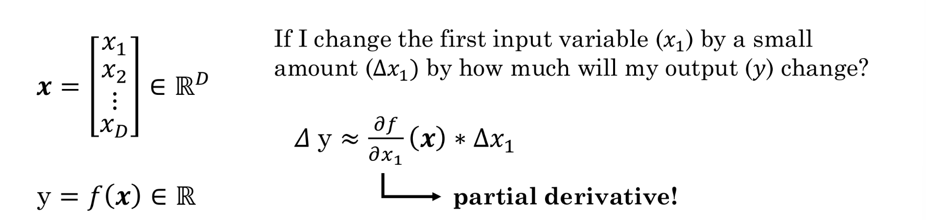
As shown in the figure above, we have an input vector x containing D features, and an output y that is a real number — the value we want to predict (e.g., the house price).

Now, let us focus on the specific question: "If I change the first input variable (x₁) by a very small amount (Δx₁), how much will my output y change?"

The tool for measuring this small change is the partial derivative:

\[ \Delta y \approx \frac{\partial f}{\partial x_1}(\mathbf{x}) \cdot \Delta x_1 \]

Let us interpret this formula:

• Δy: The change in output y (e.g., the increase in house price).
• Δx₁: The small change in input x₁ (e.g., 1 additional square meter of area).
• ≈: The "approximately equal to" sign. Since this formula is a linear approximation, when Δx₁ is very small, the approximation is very accurate.
• ∂f/∂x₁: This is the partial derivative.

The partial derivative is the core tool for measuring a function's sensitivity.

Its intuitive meaning is: the rate of change of output y with respect to input x₁, while holding all other input variables (x₂, x₃, ...) fixed.

Returning to the house price example: ∂f/∂x₁ (where x₁ is area) represents, with all other conditions (number of bedrooms, location, etc.) held constant, how much the price changes per unit increase in area.

If the computation yields ∂f/∂x₁ = 5000, it means that, all else being equal, each additional square meter of area increases the price by approximately 5000 units. This 5000 is the "sensitivity" of the price to area.

In summary, if we want to understand the relationship between changes in input x and output y, we need to know the function's response (sensitivity) to changes, and the partial derivative is the mathematical tool for measuring this sensitivity. The partial derivative tells us how the output reacts when we slightly adjust a particular input.

Why is this critical for machine learning? Because the process of "training" a model is essentially about repeatedly computing the partial derivatives of the loss function (a function that measures how inaccurate predictions are) with respect to the model's internal parameters. Through these partial derivatives, we know how to fine-tune each parameter so that the model's predictions become more accurate. This process is the core of the famous gradient descent algorithm.

---

Chain Rule

Imagine that going directly from a pixel-filled image (input x) to determining it contains a "dog" (output y) is extremely difficult. The model must bridge an enormous cognitive gap.

So this section proposes that we can decompose this complex task into two simpler, relay-like tasks:

Step 1 (performed by f₁, g₁, h₁): Feature Extraction

• Goal: Transform the raw, messy, hard-to-understand data into meaningful, structured "features." This is the most critical and remarkable part of the entire process.
• Examples:

• Image: The input is a large collection of pixel values. The job of f₁ is not to look at pixels directly, but to "learn" to identify key image features from them, such as:

  • Edges and contours
  • Object textures (e.g., a furry appearance)
  • Specific shapes (e.g., dog ears, cat noses)
  • Text: The input is a string of words. The job of g₁ is to extract text features, such as:
  • Whether it contains keywords like "urgent," "money," or "winner"
  • Whether the tone is commanding or pleading
  • Whether there are unusual capitalizations or spelling errors
  • Tabular: The input consists of several independent columns of numbers. h₁ can learn to combine these numbers into more meaningful tabular features, such as:
  • "Price per square meter" (total price divided by area)
  • "Bedroom-to-bathroom ratio"
  • Converting the location "Berkeley" into a specific risk or value index

Step 2 (performed by f₂, g₂, h₂): Decision Making Based on Features

• Goal: Now the second-step function receives the high-quality "features" processed by the first step, making its task much simpler.
• Examples:
• Image: f₂ no longer looks at raw pixels but at the features passed to it by f₁. When it sees features like "furry texture," "floppy ears," and "wet nose," it can easily determine the result is "dog."
• Text: g₂ receives features such as "contains money-related words" and "urgent tone," and can judge with high probability that this is "spam."
• Tabular: h₂ uses the various combined features computed by h₁ and then applies a relatively simple model (such as linear regression) to calculate the final price "$1,200,000."

This divide-and-conquer philosophy was traditionally carried out manually by human experts (data scientists) in a process called "feature engineering." The question marks next to f₁, g₁, h₁ in the slide hint that in modern deep learning, the model can automatically "learn" from data which features are most useful. We do not need to tell the model to look for ears and noses — it will discover on its own during training that these are key features for distinguishing dogs from cats.

This y = f₂(f₁(x)) structure is, in fact, the simplest form of a neural network. f₁ can be viewed as the earlier layers of the network (responsible for feature extraction), and f₂ as the final layer (responsible for classification or regression). A "deep" neural network simply further decomposes f₁ into more layers, learning increasingly complex features from low-level (edges) to high-level (object parts).

With this idea in mind, we unify all the separate functions from different stages and examine their sensitivity holistically. In mathematics, we can accomplish this with the chain rule.

The essence of the chain rule is: total sensitivity = sensitivity of the first stage × sensitivity of the second stage.

For a composite function:

\[ \mathbf{x} = \begin{bmatrix} x_1 \\ x_2 \\ \vdots \\ x_D \end{bmatrix} \in \mathbb{R}^D \]

\[ y = f_2(f_1(\mathbf{x})) \in \mathbb{R} \]

We obtain:

\[ \Delta y \approx \frac{\partial}{\partial x_1} f_{2}(f_{1}(\mathbf{x})) \cdot \Delta x_1 \]

\[ \Delta y \approx \frac{\partial f_{2}}{\partial x_{1}}(f_{1}(\mathbf{x})) \cdot \frac{\partial f_{1}}{\partial x_1}(\mathbf{x}) \cdot \Delta x_1 \]

Let us break down this formula:

• Δx₁: still the same small perturbation we apply to input x₁.
• Δy: the resulting change in the final output y.

The product of the two partial derivatives in the middle represents the "two-stage sensitivity":

• ∂f₁/∂x₁: Sensitivity of the first stage.

  • It measures: How sensitive is the intermediate feature f₁ to the original input x₁?
  • Example: In image recognition, if we brighten a certain pixel x₁ slightly, how much more prominent does the "detected dog ear" feature f₁ become?
  • ∂f₂/∂f₁: Sensitivity of the second stage.
  • It measures: How sensitive is the final output y to the intermediate feature f₁?
  • Example: If the "dog ear" feature f₁ becomes slightly more prominent, how much does the model's final probability of classifying it as "dog" (y) increase?

Multiplying these two sensitivities gives us the total sensitivity of y to x₁.

Modern machine learning's most important paradigm — deep learning — is essentially an objective function composed of very many stages. Each stage corresponds to a layer of the neural network, and the whole thing is essentially a very long composite function: y = f_n(...f₂(f₁(x))...).

When we train the network and find that the model's predictions have errors, we need to fine-tune thousands of parameters to reduce the error. But how do we know which ones to adjust and by how much?

The answer lies in the chain rule. An algorithm called backpropagation is, at its core, the application of the chain rule. Starting from the last layer, it computes layer by layer, in reverse, the partial derivatives (sensitivities) of the error with respect to the parameters at each layer.

• These partial derivatives tell us: "If you increase this parameter slightly, the final error will decrease/increase by this much."
• With this information, the model knows how to adjust all of its parameters to make better predictions next time.

Therefore, the chain rule is the mathematical engine that drives learning and optimization in all deep learning models.

Earlier we discussed the multiplicative single-chain case y = f₂(f₁(x)); for tasks where multiple paths converge, we can also apply the chain rule in an additive form:

\[ \frac{\partial}{\partial x} f\!\big(g(x) + h(x)\big) = \frac{\partial f}{\partial g} \cdot \frac{dg}{dx} + \frac{\partial f}{\partial h} \cdot \frac{dh}{dx} \]

---

Probability Perspective

Bayes' Theorem

Many machine learning (ML) problems can be viewed as probability problems, and Bayes' theorem is a powerful tool for solving them.

The core formula of Bayes' theorem is:

\[ P(Y = k \mid X = x) = \frac{P(X = x \mid Y = k) P(Y = k)}{P(X = x)} \]

Let us break down each term:

• \(P(Y = k \mid X = x)\): Posterior probability. This is the result we most want to know. It means: "Given the observed data features \(X=x\), what is the probability that the label \(Y\) we want to predict is class \(k\)?"

  • Example: After seeing the content of an email (\(X=x\)), what is the probability that it is spam (\(Y=spam\))?
  • \(P(X = x \mid Y = k)\): Likelihood. It means: "If the label Y is definitely class k, what is the probability that we observe data features X=x?"
  • Example: In an email confirmed to be spam (\(Y=spam\)), what is the probability of seeing words like "Nigeria" and "urgent need for money" (\(X=x\))? This probability is typically easier to compute than the posterior directly.
  • \(P(Y = k)\): Prior probability. This is our initial judgment or belief about the probability that label Y is class k, before observing any data.
  • Example: Based on historical data, we know that about 30% of all emails are spam, so \(P(Y=spam)=0.3\).
  • \(P(X = x)\): Evidence. This is the total probability of observing features X=x, regardless of the label.

That is:

\[ \text{Posterior} = \frac{\text{Likelihood} \times \text{Prior}}{\text{Evidence}} \]

To put it simply, if we use "overcast skies to predict whether it will rain":

• Posterior probability: after seeing the overcast sky, your updated belief about whether it will rain today
• Likelihood: if it is indeed going to rain, how likely is it that the sky would be overcast
• Prior probability: before seeing the sky, based on experience, the probability of rain on any given day
• Evidence: regardless of whether it rains, how likely is it for the sky to be overcast today

Since directly computing the posterior probability \(P(Y=k \mid X=x)\) is often difficult, in most cases estimating the likelihood \(P(X=x \mid Y=k)\) and the prior probability \(P(Y=y)\) is much easier.

That still leaves the evidence. We typically obtain the evidence through the law of total probability:

Law of total probability:

\[ P(X = x) = \sum_{y} P(X = x, Y = y) \]

\[ = \sum_{y} P(X = x \mid Y = y) P(Y = y) \]

In many cases — for example, when determining whether an email is spam — we compare \(P(Y=spam \mid X=x)\) with \(P(Y = not\_spam \mid X = x)\). Since both share the same denominator \(P(X=x)\), we only need to compare the numerators: whichever numerator is larger corresponds to the class with the higher posterior probability. This is why, in many classification algorithms (such as Naive Bayes), the core computation involves calculating and comparing (likelihood × prior), while ignoring the evidence.

Of course, if you need an exact value — such as "the probability that this email is spam is 98.3%" — then you must compute the evidence using the law of total probability and perform the division.

Supervised Learning Pipeline

In the vast majority of cases, when people refer to "machine learning," they mean supervised learning. Reinforcement learning, clustering, and other paradigms are typically stated explicitly.

Below is an overview of a typical supervised learning training pipeline.

The core idea of supervised learning is quite intuitive: we believe there exists an underlying pattern between inputs and outputs (the true function \(F\)), and we want to use a collection of examples (training data) to find a model (approximate function \(f\)) that mimics and approximates this unknown pattern. In other words: the essence of supervised learning is function approximation:

• Function approximation: Learn a function \(f: X \to Y\) from an input space \(X\) (observation set) to an output space \(Y\) (target set), using a set of labeled training examples \(D_{\text{train}} = \{(x_1, y_1), \dots, (x_N, y_N)\}\).
• Generalization: Ideally, the learned function \(f\) also performs well on test data not included in the training set \(D\).
• Example: Image classification.

Using house price prediction as an example:

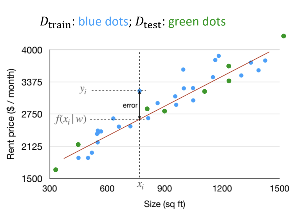
(1) Dataset:

• Training data \(D_{train}\), shown as blue dots in the figure, used for learning the model
• Test data \(D_{test}\), shown as green dots in the figure, used for evaluating the model's generalization capability

(2) Model:

Our goal is to fit a straight line describing the relationship between area and rent:

• Model function: \(f(\mathbf{x}|\mathbf{w}) = \mathbf{w}^{\mathbf{T}} \mathbf{x}\)
• \(\mathbf{x}\) is the input feature vector
• \(\mathbf{w}\) is the weight vector — the object we need to learn

(3) Learning Process: Loss Function

• Training objective: For every data point \((x_i, y_i)\) in the training set, we want the model's prediction \(f(x_i | \mathbf{w})\) to be as close as possible to the true value \(y_i\)
• To measure the quality of a single prediction, we use squared loss to compute the square of the difference between the true value and the predicted value: \(L(y, y') = (y - y')^2\)

For the entire dataset, we can compute the average squared loss across all samples:

\[ MSE = \frac{1}{N} \sum_{i=1}^{N} (y_i - \hat{y}_i)^2 = \frac{1}{N} \sum_{i=1}^{N} L(y_i, \hat{y}_i) \]

(4) Learning Objective:

Our goal is to find the optimal set of weights that minimizes the total loss across the entire training set. Expressing this as an optimization problem:

\[ \underset{\mathbf{w}}{\operatorname{argmin}} \sum_{i \in D_{\text{train}}} L(y_i, f(\mathbf{x}_i \mid \mathbf{w})) \]

The above is a template using a general loss function L, meaning: find the weight vector \(\mathbf{w}\) that minimizes the sum of losses over all training samples. That is, the true value of the i-th sample \(y_i\) is fed in, the model's prediction for the i-th sample \(f(\mathbf{x}_i \mid \mathbf{w})\) is obtained, and then the difference between these two inputs is compared to output a numerical value representing the magnitude of the loss or error. Applying this to our example:

\[ \text{Objective}(\mathbf{w}) = \min_{\mathbf{w}} \frac{1}{N} \sum_{i \in D_{\text{train}}} L(y_i, f(\mathbf{x}_i \mid \mathbf{w})) \]

Substituting in the loss function:

\[ \text{Objective}(\mathbf{w}) = \min_{\mathbf{w}} \frac{1}{N} \sum_{i=1}^{N} (y_i - f(\mathbf{x}_i \mid \mathbf{w}))^2 \]

In other words, our learning objective is to make the model perform as well as possible across the entire training set. This is typically achieved by minimizing the Sum of Squared Errors (SSE), which is mathematically equivalent to minimizing the Mean Squared Error (MSE).

(5) Optimization:

To achieve the learning objective, we can find the loss-minimizing weight vector through various methods, generally including:

• Closed-form Solution
• Gradient Descent (GD)
• Stochastic Gradient Descent (SGD)

Additionally, several techniques have been developed to improve the optimizer (details in the deep learning notes):

• Adaptive Gradient
• Momentum
• Learning Rate
• Regularization

(6) Generalization:

The purpose of training a model is for it to perform well on unseen data; otherwise, training is meaningless. In other words, the model should also achieve low total loss on the test set. If the model performs well on the training set but poorly on the test set — i.e., test error >> training error — then we have overfitting. If the model performs poorly on both the training set and the test set, then we have underfitting.

Generalization faces challenges such as interpolation vs. extrapolation and domain shift.

If we analyze the generalization error of a machine learning model theoretically, we generally decompose it into three main components:

• Bias: the gap between the model's average prediction and the true value. High bias means the model's fundamental assumptions are wrong — it cannot even fit the basic patterns in the data, so adding more data will not help.
• Variance: how much the model's predictions fluctuate when trained on different datasets. High variance means the model is overly sensitive to the training data — small changes in the training data cause dramatic changes in the model, i.e., the model has learned too much of the noise and idiosyncrasies in the training data.
• Noise / Irreducible Error: the error caused by inherent noise in the data itself. This is the lower bound of error that no model can eliminate.

In general, underfitting is caused by high bias — the model's complexity is too low to capture the underlying complex patterns in the data. Overfitting is caused by high variance — the model's complexity is too high, and it learns not only the true patterns but also the noise in the training data as if it were a pattern. Therefore, the goal is typically to find a balance that minimizes overall bias and variance. In traditional machine learning, this balance can generally be found by minimizing (bias² + variance). However, this phenomenon no longer holds for modern large-scale models — this is the double descent phenomenon. Double descent challenges our traditional understanding of overfitting and reveals why today's massive models, whose parameter counts far exceed the number of training samples, can still perform excellently. Under this new regime, larger, more complex models actually perform better and exhibit stronger generalization capability.

(7) Evaluation:

Different machine learning tasks require different metrics for evaluation.

Regression Tasks — predicting continuous values:

• MAE (Mean Absolute Error): the average of the absolute differences between predicted and true values
• MSE (Mean Squared Error): the average of the squared differences between predicted and true values; it amplifies the effect of large errors and is more sensitive to outliers
• RMSE (Root Mean Squared Error): the square root of MSE; this is the most commonly used regression metric
• \(R^2\) (R-squared): indicates the extent to which the model's predictions explain the variation in the actual data. Values range from 0 to 1, with values closer to 1 indicating better fit.

Classification Tasks — predicting discrete categories:

• Confusion Matrix: a matrix formed by predicted positive/negative vs. actual positive/negative; the following metrics are all derived from this matrix:
• Accuracy: note that this metric can be highly misleading with imbalanced data (e.g., 99% of emails are not spam)
• Precision: important when the cost of false positives is high, e.g., in spam filtering we do not want to incorrectly classify important emails as spam
• Recall / Sensitivity: important when the cost of false negatives is high, e.g., in cancer diagnosis we do not want to miss any truly positive patient
• F1-Score: the harmonic mean of precision and recall; F1 is high only when both are high
• AUC: area under the ROC curve; measures the model's ranking ability and is, in many scenarios, a more stable performance metric than accuracy

Cross-Validation (CV):

• If the dataset is small, the train-validation-test split may yield unstable evaluation results due to randomness
• CV divides the training data into K folds, and in each round uses K-1 folds for training and the remaining fold for validation. After repeating K times, the average of the K evaluation scores provides a more robust and reliable estimate of model performance.

(8) Theoretical Justification for Loss Function Selection (not required for engineering practice)

Above, we naturally used a straight line to approximate the house price prediction model, then used MSE to compute the average squared loss across all samples as our measure of loss — that is, the loss function. The choice of MSE as the loss function for linear regression is not arbitrary; it has a theoretical justification grounded in the probabilistic approach and maximum likelihood estimation.

First, we must acknowledge a fact: no model can perfectly predict the real world. Even if we use a line \(f(\mathbf{x}|\mathbf{w})\) to predict house prices, there will always be a residual error \(\epsilon\) between the true value \(y\) and the predicted value \(f(\mathbf{x}|\mathbf{w})\), i.e., \(y=f(\mathbf{x}|\mathbf{w})+\epsilon\).

Now we make a key assumption: we assume this error \(\epsilon\) is not completely random and lawless, but follows a normal distribution with mean zero (a very reasonable assumption, as it is extremely common in the real world). Under this assumption, we can re-describe our model from a probabilistic perspective:

For a given input \(\mathbf{x}\), the probability distribution of the output \(y\) is a normal distribution centered on the line's predicted value \(f(\mathbf{x}|\mathbf{w})\).

Now we have a collection of training data \((x_1,y_1),(x_2,y_2),...\), and we can apply maximum likelihood estimation (MLE):

What kind of line (i.e., what parameters w) should we choose so that the probability of observing the data we actually have is maximized? In other words, the best line must be the one that best explains our existing data.

Given the normal distribution assumption, the probability of observing a single data point \(y_i\) is:

\[ P(y_i \mid \mathbf{x}_i; \mathbf{w}) \propto \exp\left( -\frac{(y_i - f(\mathbf{x}_i \mid \mathbf{w}))^2}{2\sigma^2} \right) \]

By the MLE principle, we want to maximize the total probability of observing all data points. This total probability (the likelihood function) is the product of all individual probabilities:

\[ \text{Likelihood}(\mathbf{w}) = \prod_{i=1}^{N} P(y_i \mid \mathbf{x}_i; \mathbf{w}) \]

For computational convenience, we maximize the log-likelihood instead, which yields the same optimal w as maximizing the original likelihood. Taking the log turns the product into a sum:

\[ \begin{align*} \log\left(P(y_i \mid \mathbf{x}_i; \mathbf{w})\right) &= \log\left[ \frac{1}{\sqrt{2\pi\sigma^2}} \exp\left( -\frac{(y_i - f(\mathbf{x}_i \mid \mathbf{w}))^2}{2\sigma^2} \right) \right] \\[8pt] &= \log\left(\frac{1}{\sqrt{2\pi\sigma^2}}\right) + \log\left[ \exp\left( -\frac{(y_i - f(\mathbf{x}_i \mid \mathbf{w}))^2}{2\sigma^2} \right) \right] \\[8pt] &= \log\left(\frac{1}{\sqrt{2\pi\sigma^2}}\right) - \frac{(y_i - f(\mathbf{x}_i \mid \mathbf{w}))^2}{2\sigma^2} \end{align*} \]

This is the simplified form of the log-likelihood for a single sample. Our learning objective is to maximize the log-likelihood over the entire dataset, so we sum over all samples and distribute the summation to each term:

\[ \sum_{i=1}^{N} \left[ \log\left( \frac{1}{\sqrt{2\pi\sigma^2}} \right) - \frac{(y_i - f(\mathbf{x}_i \mid \mathbf{w}))^2}{2\sigma^2} \right] \]

\[ = \sum_{i=1}^{N} \log\left( \frac{1}{\sqrt{2\pi\sigma^2}} \right) - \sum_{i=1}^{N} \frac{(y_i - f(\mathbf{x}_i \mid \mathbf{w}))^2}{2\sigma^2} \]

\[ = N \log\left( \frac{1}{\sqrt{2\pi\sigma^2}} \right) - \frac{1}{2\sigma^2} \sum_{i=1}^{N} (y_i - f(\mathbf{x}_i \mid \mathbf{w}))^2 \]

Since our goal is to find the weights w that maximize the above expression, the left half of the expression is irrelevant to the result — it is a constant with respect to finding the optimal w. The coefficient on the right is an ordinary constant, and the squared terms are positive, so we can convert the optimization objective to:

\[ \underset{\mathbf{w}}{\operatorname{argmax}} \left[ \text{constant} - \text{positive constant} \cdot \sum_{i=1}^{N} (y_i - f(\mathbf{x}_i \mid \mathbf{w}))^2 \right] \]

This objective is completely equivalent to:

\[ \min_{\mathbf{w}} \sum_{i=1}^{N} (y_i - f(\mathbf{x}_i \mid \mathbf{w}))^2 \]

Thus, through the probabilistic approach and maximum likelihood estimation, we have mathematically proven that the optimal loss function for linear regression is minimizing the total squared loss (MSE).

---

Let us look at applications of supervised learning in robotics:

1. Training Dataset

   • Formula: \(D_{train} = \{(x_1, y_1), \cdots, (x_N, y_N)\}\)
   • \(x\) (input): The robot's sensor data (e.g., images) or its own state (e.g., joint angles).
   • \(y\) (output/label): The "correct answer" the robot needs to learn. 2. Different meanings of \(y\)
   • Dynamics: \(y\) represents the "outcome" of an action (e.g., the robot's next state). This is important for model-based control and reinforcement learning (RL).
   • Action: \(y\) represents "the correct action to execute." This is the core of imitation learning. 3. Core Challenges
   • How to generate high-quality training data (\(y\)).
   • How to effectively apply the learned model to robot control.

The core of supervised learning for robotics is decomposing a complex system into a known part and an unknown part, then using machine learning to approximate the unknown part:

\[ \dot{x} = f_n(x, u) + f(x, c(t)) \]

• \(\dot{x}\): The rate of change of the system state (e.g., velocity and angular velocity).
• \(f_n(x, u)\): The known, idealized physical model (nominal model). For example, the dynamics in a wind-free, drag-free environment.
• \(f(x, c(t))\): The unknown, hard-to-model "residual term." For example, wind, water drag, friction, etc.

Through supervised learning, a model is trained to accurately predict this unknown residual term \(f(x, c(t))\).

• Input (\(x_{train}\)): The robot's current state \(x\).
• Output (\(y_{train}\)): The residual measured in the real world, i.e.: \(y = \dot{x}_{\text{real}} - f_n(x, u)\)

---

Example 1: Drone flying through hoops in windy conditions

• Challenge: Wind force \(f(x, c(t))\) is an unknown disturbance that causes the drone to deviate from its planned trajectory.
• Solution:
  1. The drone has a base controller built on the known model \(f_n\).
  2. By flying in windy conditions and collecting data, a "wind prediction model" is learned to estimate \(f\).
  3. The final controller combines the known model \(f_n\) with the learned residual model \(f\), enabling it to actively compensate for wind and achieve precise control.

Example 2: Robotic arm grasping objects underwater

• Challenge: Buoyancy and viscous drag from water \(f(x, c(t))\) are unknown factors not accounted for in the in-air model \(f_n\).
• Solution:
  1. Collect data underwater and compute the "residual forces" caused by water \(f\).
  2. Train a neural network to learn this residual force model.
  3. During deployment, the controller uses the known model \(f_n\) and adds the compensating forces predicted by the learned model \(f\) to counteract the underwater environment's effects, achieving precise grasping.

Limitations of ML

Machine learning's reliance on learning from data inherently imposes limitations:

1. Data limitations: robotics ML, for instance, has progressed slowly due to insufficient data
2. Generalization limitations: it remains difficult to make machines generalize as effortlessly as humans do
3. Structural limitations: the paradigm \(f=ML(D)\) means machine learning can perform very well on specific tasks, but struggles with few-shot learning

---

评论