Deep Learning

A New Brief History of Deep Learning

After studying deep learning for some time, I have reorganized a new version of the brief history of deep learning based on my own understanding.

The Afterglow of a Golden Age

As early as the 1980s, Bell Labs had developed early neural network hardware prototypes. These prototypes were the ancestors of modern AI chips (such as Google TPUs and NVIDIA GPUs). Researchers at the time attempted to simulate neural network operations directly on silicon through circuits, rather than running them solely through software.

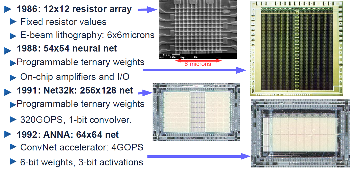
Among these, the Net32k developed in 1991 achieved a performance of 320 GOPS (billions of operations per second), an astonishing speed at the time. It contained a 1-bit convolver specifically designed for convolution operations, the core algorithm of modern visual AI.

ANNA, developed in 1992, was a dedicated ConvNet (Convolutional Neural Network) accelerator. The renowned AI pioneer Yann LeCun was working at Bell Labs at the time. The ANNA chip was developed specifically to accelerate the convolutional neural networks he designed (such as LeNet for recognizing check digits).

Starting in 1993, check-reading systems based on convolutional neural networks (ConvNets) began commercial deployment in ATMs across the United States and Europe. By the late 1990s, approximately 10% to 20% of all checks in the U.S. were processed by this system. Inside the ATMs, these algorithms did not run on general-purpose processors but on DSP (Digital Signal Processor) cards plugged into PCs. The initial chip used was AT&T's DSP32C, the first 32-bit floating-point DSP at the time, with impressive computational power. Although large-scale commercial deployment relied more on mature DSP technology, ANNA proved the feasibility of accelerating AI computations through custom hardware (similar to today's NPUs). The convolutional neural networks used in these systems (such as LeNet-1) were trained in a Lisp-based simulation environment called SN. After training, researchers used a "compiler" to convert them into C code that ran directly on the hardware.

The hardware we see from Bell Labs during 1986-1996 was, in fact, the afterglow of America's last era of "no-cost-spared, no-return-expected" laboratory research.

However, the technology that ultimately provided the massive computational power for AI training was NVIDIA's GPUs. In the mid-2000s, some researchers (such as Ian Buck at Stanford) discovered that GPUs originally designed for playing Half-Life or World of Warcraft had a natural advantage in matrix operations. Jensen Huang, despite years of losses at NVIDIA, pushed forward the CUDA architecture against Wall Street pressure, transforming GPUs from gaming tools into general-purpose computing platforms. The success of AlexNet was largely due to its two students (Alex and Ilya) who hand-wrote efficient CUDA kernel code, reducing training time from months to days. In the 2012 ImageNet competition, AlexNet crushed the second-place entry using just two NVIDIA graphics cards, achieving training results far surpassing the capabilities of laboratory clusters.

Scholars in Exile

It is well known that AI development went through several winters. Before AlexNet's breakthrough in 2012, neural network research was in a so-called "AI winter," and the American academic mainstream was even somewhat hostile toward the field.

Kunihiko Fukushima proposed the Neocognitron in 1979. It was the first true multi-layer convolutional neural network in history. Yann LeCun later acknowledged that his LeNet (the algorithm running on the hardware shown in the earlier images) was largely inspired by Fukushima's ideas of "receptive fields" and "hierarchical structures."

However, ever since the publication of Perceptrons, neural networks had been relentlessly bullied by the academic mainstream. In 1969, MIT's AI titan Marvin Minsky (a representative of symbolic AI) published Perceptrons, mathematically proving that a single-layer neural network could not even implement the simple XOR logic. This book directly triggered the first AI winter, lasting a full decade. The later efforts of Hinton and others were essentially a forty-year battle against the ghost of Minsky's "neural networks are useless" thesis.

Geoffrey Hinton left Carnegie Mellon University for the University of Toronto in 1987, dissatisfied with U.S. military funding of research. In the United States, funding agencies like DARPA typically demanded "immediate military or commercial returns." If neural networks failed to produce breakthroughs for five consecutive years, funding would be cut. CIFAR (the Canadian Institute for Advanced Research) made a remarkably visionary move in 2004 by funding the "Neural Computation" project established by Hinton. They gave Geoffrey Hinton a modest but extraordinarily unrestricted grant that required no commercial outcomes—only that Hinton organize intimate symposia of top scholars every few months. This established an "underground network of rebels." Hinton, Bengio, LeCun, and others regularly met in Canada, bolstering each other's spirits. They called themselves the "NCAP" (Neural Computation and Adaptive Perception) group.

European researchers led the way in neural networks for handling "memory" and "logic." Jurgen Schmidhuber worked at the IDSIA laboratory in Lugano, Switzerland. He and his student Sepp Hochreiter invented LSTM (Long Short-Term Memory) in 1997. Before the advent of Transformers, LSTM was the undisputed global champion for speech recognition (Siri, Google Translate) and natural language processing. In Switzerland and Germany, the academic system differs drastically from the United States. Laboratories like Jurgen Schmidhuber's had very stable government funding. Professors enjoyed great autonomy—even if the entire world considered neural networks garbage, a professor could still spend twenty years exploring them with students. Moreover, the European mentorship tradition strongly emphasizes continuity. This environment allowed them to delve into extremely abstract mathematical problems (such as the vanishing gradient problem solved by LSTM), without being forced, like American doctoral students, to chase the hottest research directions (such as SVMs at the time) in order to find jobs.

One might assume that American scientific research is highly free. However, research funding at top U.S. universities is heavily dependent on the NSF (National Science Foundation) and DARPA (Defense Advanced Research Projects Agency). Their money typically comes with clear mission objectives. If a research direction (such as neural networks) fails to produce notable results—like recognizing tanks or translating documents—within ten years, funding is swiftly cut. In the United States, junior faculty (Assistant Professors) face the pressure of the "Tenure Track." If your research field produces no results and you cannot publish in top journals within six years, you pack your bags and leave. This drives American academia toward "fast-result" fields (such as the mathematically more rigorous SVMs at the time).

Meanwhile, the U.S. suffered from severe mainstream bullying. Another prerequisite for free research is peer review, which in the 1990s became a kind of "soft shackle" in America. When the mainstream academic establishment (MIT, Stanford, etc.) deemed neural networks a "dead end," any paper on neural networks struggled to get published at top conferences. In the United States, because the academic community is extremely active and competitive, "non-mainstream" work has difficulty obtaining resources. In Canada and Europe, because academic circles were relatively independent, they inadvertently created "safe havens" where heterodox ideas could survive. Once the academic establishment formed a consensus, this "freedom" turned into a tyranny of consensus.

Under this tyranny, around 2004-2006, Hinton keenly realized that if they did not rebrand, their papers would not even reach reviewers. So he proposed "Deep Belief Networks" and used "greedy layer-wise unsupervised pre-training" to solve the problem of training deep networks at the time. It was this rebranding that formally replaced the notorious terms "multilayer perceptron" and "artificial neural network" with "Deep Learning," successfully bypassing the aesthetic fatigue of academic committees through a "reskin."

In the 2020s, even as OpenAI went closed-source and three major American AI companies poured trillions of dollars into training AI, they still could not leave Chinese companies and research institutions completely behind. This is precisely because both the United States and China are fundamentally hyper-utilitarian. The American research environment resembles a brutally efficient secondary market: when a direction (such as generative AI today, or SVMs back then) shows potential for profit or top-journal publications, all resources (talent, computing power, funding) flood in like a frenzy, creating overwhelming advantages. Conversely, when a direction is in a "value trough" (like neural networks in the 1990s), it is quickly liquidated. This "winner-take-all" logic makes it very difficult for America to tolerate long-term "cold" research fields that do not produce results.

From 1990 to 2010, the neural network community was very small—its members were not just peers, but comrades-in-arms. Hinton firmly believed that since the human brain is composed of neurons, simulating neurons must be the only path to achieving intelligence. He once joked: "If you think neural networks don't work, it's because your model isn't big enough, or your data isn't sufficient—it's definitely not that the theory is wrong." When Yann LeCun's funding was cut at Bell Labs in the U.S. due to the parent company's bankruptcy and restructuring, Hinton would invite him to Canada for exchanges, or find ways to support each other in academic evaluations. They even joked about being the "Neural Network Mafia," because they were trying to force open a crack in an academic world dominated by mainstream statistics. During that period, their students had great difficulty finding faculty positions at top universities, and many brilliant minds were forced to change careers.

On the day AlexNet won in 2012, Hinton did not display wild excitement backstage. He simply said to his students calmly: "We told them (the academic world) that this works. Now they finally believe us."

Another scholar in exile was Yoshua Bengio. Compared to LeCun and Hinton, who moved between industry and elite universities, Bengio was more of an ascetic. He steadfastly remained at the University of Montreal (even when funding there was extremely scarce) and refused nearly all full-time, high-salary offers from major tech companies. His contributions to sequence modeling and generative models (the foundations for later GANs and word embeddings) were decisive. He was the purest academic banner-bearer of this "Mafia."

In 2018, Hinton, LeCun, and Bengio jointly received the Turing Award.

In addition to the famous exiles mentioned above, there was another important one—Fei-Fei Li. After immigrating to the United States from Chengdu at age 15 with her parents, her life was far from easy. To support her family, she worked in restaurants. At the most difficult times, she took out a loan to open a dry-cleaning shop to cover the family's expenses. Even while studying as an undergraduate at Princeton and as a doctoral student at Caltech, she returned every weekend to the dry-cleaning shop in New Jersey to help her parents. This background kept her grounded and at a distance from "purely academic" discourse. For her, scientific research was not a game in an ivory tower, but an extraordinarily precious dream that had to be defended with every ounce of effort.

The reason AlexNet became an overnight sensation in 2012 was that it dominated the ImageNet competition. The creator of ImageNet, Fei-Fei Li, firmly believed in the late 2000s: "If algorithms are the engine, data is the fuel." While all of America was researching elegant SVM algorithms, she was doing the dirtiest, most laborious work—cleaning millions of internet images.

In the late 2000s, the explosion of social media platforms (Flickr, Facebook) produced the first massive, naturally annotated image datasets in human history. Previously, Bell Labs could only process checks (a specific scenario) because there simply were not hundreds of millions of photos of cats and dogs for models to learn from. The growth of the internet inadvertently prepared all the fuel that deep learning needed.

Although Fei-Fei Li was not marginalized for supporting neural networks, she was marginalized for insisting that data was more important than algorithms. The academic mainstream at the time (most labs at MIT, Stanford, etc.) was focused on more elegant mathematical models (such as SVMs), believing that improving AI performance should rely on humans writing smarter feature-engineering code.

When Li began working on ImageNet, many peers privately mocked her: "This assistant professor is crazy—she's doing the most technically trivial work of 'labeling.'" When ImageNet's first poster was presented at the top conference CVPR in 2009, almost no one paid attention; everyone thought it was just a large but useless database. This research direction could not secure major funding from mainstream sources (NSF, etc.) at the time. She even had to resort to layoffs and dip into her personal funds to pay the data annotators (workers on Amazon's crowdsourcing platform).

Although Fei-Fei Li was not part of the "Neural Network Mafia's" original inner circle, she ultimately became their greatest ally. If Hinton's camp was convinced that the "internal combustion engine" (neural networks) would definitely work, then Li was the person convinced that "without oil (massive data), even the best engine is just scrap metal." In 2012, the reason AlexNet won the ImageNet competition was essentially that "a fallen theory" met "neglected fuel." At that moment, these two "non-mainstream" forces converged, truly inaugurating the modern era of AI.

The Age of Exploration

AlexNet's stunning leap in 2012 not only shattered the silence of the academic world but blasted open a breach in the stagnant old order. If the period before 2012 was the "Mafia's" guerrilla war behind enemy lines, then after 2012, AI entered a grand, sweeping, almost religiously fervent "Age of Exploration."

In 2015, He Kaiming (Kaiming He), then at Microsoft Research Asia, proposed ResNet (Residual Network). Before this, neural networks deeper than 20 layers could not be trained due to the "vanishing gradient" problem. He Kaiming brilliantly introduced a "shortcut" (Skip Connection), allowing information to pass across layers without loss. ResNet pushed the number of layers directly to 152 and even thousands. This was not merely a technical breakthrough but an engineering philosophy: If you cannot solve complexity, give complexity a way through.

In 2016, DeepMind's AlphaGo defeated Lee Sedol in Seoul. This was not just a Go program's victory—it demonstrated for the first time to the general public that Deep Learning (DL) + Reinforcement Learning (RL) could produce something remarkably close to "intuition." That night, elites around the world began to experience collective anxiety, and capital began flooding into Silicon Valley like a tidal wave.

During this period, Google's researchers inadvertently gave the world one of its most momentous gifts, while also sowing the seeds of their own "brain drain." In 2017, eight researchers at Google Brain published the epoch-making paper "Attention is All You Need." They dethroned the RNN and LSTM (what Schmidhuber had spent twenty years perfecting), which had long dominated sequence modeling, and proposed the Transformer. Rather than reading "left to right" like a human, it used an attention mechanism to achieve global, concurrent perception. Ironically, all eight authors left Google after the paper's publication, going on to found companies such as Character.ai, Cohere, and Essential AI. This marked the definitive shift of AI's center of innovation from "established laboratories" to "unicorn startups." AI was no longer a bonsai in the lab—it was a great vessel about to set sail.

Around 2020, a qualitative shift occurred in the academic landscape. People stopped debating elegant algorithmic architectures and instead embraced "Scaling Laws." Ilya Sutskever, then Chief Scientist at OpenAI (and Hinton's prized student), firmly believed: as long as the model is large enough and the data plentiful enough, intelligence will "emerge." The release of GPT-3 in 2020 validated this hypothesis. It no longer required fine-tuning for specific tasks but demonstrated astonishing generalization capabilities.

If in 2009 Fei-Fei Li was still manually annotating images, then by 2022, virtually all text, code, and artwork ever produced by humanity on the internet had been fed into these black boxes. Intelligence was no longer derived through deduction—it was "refined" from the ruins of human civilization (massive data).

The Imperial Age

If AlexNet in 2012 ignited the Age of Exploration, then the sudden emergence of ChatGPT in 2022 heralded that the AI race had transitioned from the chaotic Age of Exploration into a computing-power arms race among major corporations. The AI world had officially entered the Imperial Age. This transformation was not merely technological—it was a comprehensive siege of resources, computing power, and geopolitics.

In 2012, a brilliant doctoral student with two graphics cards could beat a training cluster and win a competition. By 2026, this had become a fantasy. The cost of a single training run for current Frontier Models (GPT-5 class or Claude 4 class) has crossed the $1 billion threshold. This means that without tens of thousands of NVIDIA B200 or more advanced GPUs in a computing cluster, you do not even have a seat at the table.

In the United States, large AI models quickly came to be dominated by four naval emperors:

Power	Style	"Imperial" Characteristics
OpenAI / Microsoft	Orthodox Papacy	Holds the strongest first-mover advantage and an almost religious rallying cry of "AGI," building extremely high barriers through a closed ecosystem.
Google	Fading Old Empire	Possesses the world's most complete TPU supply chain and data feedback loop. Though somewhat slow to react, it has the deepest reserves, steadfastly guarding its search and mobile strongholds.
Anthropic / Amazon	Pragmatic Knights	Pursues an extreme safety and alignment path, relentlessly focusing on the enterprise market and long-context capabilities, backed by Amazon's limitless cloud resources.
Meta	Open-Source Pirate King	Zuckerberg plays an exceptionally unique role. Through continuous open-sourcing of the Llama series, he seeks to undermine the "closed monopoly" of the other three, building free ports outside the imperial walls.

By 2026, the focus of large model competition has shifted from "GPUs" to "electricity." Microsoft and OpenAI have even begun investing in nuclear power generation (SMR, Small Modular Reactors). The end of intelligence is energy—this has become a national-level imperial strategy, no longer a purely commercial endeavor.

On the other hand, among the original four emperors, Meta, like Whitebeard, has been swept away by the tides of the era. After losing its emperor status, Meta was also in internal disarray. The fading old empire, Google, leveraged its early advantages—strong research heritage and abundant TPU computing power—to quickly reverse course, overtaking ChatGPT and reclaiming the throne. Claude, meanwhile, pivoted its strategy to specialize in coding, becoming the undisputed leader in the programming domain. The competition among four emperors evolved into a rivalry among three great powers: OpenAI's ChatGPT, Google's Gemini, and Anthropic's Claude.

Power	Flagship Model (2026 Q1)	Core Strength (Advantage)	Elo Score (LMSYS)	Imperial Role
Anthropic	Claude 4.6 Opus	God of Logic and Code. SWE-bench score 80%+, virtually a perfect "digital engineer."	1506 (Top)	Rational Papacy: Extreme safety and code logic.
OpenAI	GPT-5.2 Pro	Master of Strategy and Planning. Excels at multi-step reasoning and complex decision-making; its "chain of thought" depth is unmatched.	1498	Orthodox Royalty: Though its dominance has declined, it remains the definer of the AI world.
Google	Gemini 3 Pro	Multimodal and Long-Context Giant. Supports 5M+ context, with the world's best real-time video understanding capability.	1486	Resource Titan: Sits atop TPU computing clusters and the limitless fuel of YouTube's corpus.

Since the stunning debut of DeepSeek in 2025, a "Seven Warlords" configuration has also emerged on the global stage:

Seat	Power	Representative Model	Asymmetric Lethality (Core Feature)	Archetype
1	Meta	Llama 5	Standard-bearer of open source. Controls the PyTorch protocol; though it lost in closed-source competition, its models are the cornerstone of private deployments worldwide.	Whitebeard: Though fallen from the throne, its legacy sustains half the AI world.
2	xAI	Grok 4.1	Physical world and real-time data. Real-time connection to X platform corpus, deeply tied to SpaceX and Tesla's humanoid robot data.	Blackbeard: Wildly ambitious, forcing its way to the top through "brute-force computing."
3	Qwen (Alibaba)	Qwen 3 Max	Industrial and engineering excellence. The world's most comprehensive "full stack": long-context, multimodal, extreme coding support. The absolute hegemon of the Asian market.	Gold Emperor: Commands global commerce, ruling productivity tools with the most diligent update cadence.
4	DeepSeek	V3 / R2	A miracle of algorithmic efficiency. Achieves 90% of imperial-tier performance at 1/10 the cost. Globally recognized as an assassin in mathematical reasoning and logical efficiency.	Hawk-Eye: A solitary swordsman whose technique (algorithms) is devastatingly precise, striking exactly at the pulse of cost-efficiency.
5	Perplexity	Sonar 2.0	The terminator of search. No longer pursuing model scale, but rather the ultimate speed of information retrieval and refinement.	Jinbe: Unbeatable in its specific waters (search), deeply trusted by efficiency-minded users.
6	Mistral AI	Large 3	Sovereignty and privatization. Europe's last bastion of dignity. Elegantly designed models representing the best balance between privacy, performance, and sovereignty for enterprises.	Crocodile: Once challenged the emperors, now defending its territory with formidable barriers across Europe.
7	Cohere	Command R3	Enterprise architect. Focused on RAG (Retrieval-Augmented Generation) and agentic architectures; its models are built for processing rigorous legal and financial documents.	Moria: Though less renowned, it has spent years cultivating deep expertise in the enterprise shadow realm (RAG).

It is worth noting that although Meta has fallen from its emperor's throne, because PyTorch was originally developed by Meta—even though Meta has since donated it to the PyTorch Foundation—Meta still retains the ability to rule from behind the curtain.

The One and Only Great Treasure

If we compare AGI (Artificial General Intelligence) to the One Piece (the Great Treasure), then in 2026, we are indeed at the very climax of the Age of Exploration. Whether emperors or warlords, major corporations no longer hide their ambitions. All their computing-power races and energy scrambles are essentially a fight for the nautical chart leading to "Laugh Tale" (the AGI endpoint).

In the 2026 consensus, AGI is the ultimate weapon that would allow its possessor to "rule the world." It is no longer just a tool that writes code or generates art, but a "digital deity" capable of logical reasoning, scientific discovery, and even self-iteration at the level of a human expert. The true realization of AGI would mean human society leaping directly from an era of "labor scarcity" to one of "extreme abundance."

Before the Imperial Age began in 2022, only a few people believed that Laugh Tale truly existed. However, after ChatGPT's release in 2022 triggered a massive tsunami, from the era of four emperors to that of the three great powers and seven warlords, the entire world learned of the Great Treasure's existence. From that point on, every capable company in the world joined the race, and the seas became crowded with ships.

In 2023, the internal factional struggle at OpenAI (the Altman ousting incident) revealed that the "Great Treasure" might have already shown the tip of an iceberg (the rumored Q* algorithm). From that moment, major companies were no longer competing to "build better products"—they were fighting to "be the first to touch the divine."

However, whether the Great Treasure actually exists remains a hotly debated topic to this day. Current views on AGI fall roughly into three camps:

1. Those who firmly claim AGI is imminent, primarily including capital-driven figures like Musk and Altman.
2. Skeptics, comprising most scientists, who believe current AI is riding a bubble inflated by excessive hype. They argue that no matter how powerful LLMs become, they are fundamentally "probabilistic prediction" machines incapable of truly understanding causality. They mock current AI as being like a blind person who has read every book but never seen the world.
3. Moderates, who believe whether AGI can be achieved depends on how AGI is defined. If jagged intelligence qualifies as AGI—rather than requiring at least human-level intelligence as the standard—then AGI may indeed be achievable. This camp holds that if an AI Agent can independently complete a full day's work of a "remote employee" (i.e., a Long-horizon Agent), then it constitutes AGI. Even if it cannot weep like a human, as long as it gets the job done, it is the Great Treasure.

Clearly, merely replacing one person's job is not the ultimate goal of artificial intelligence research. Robotic arms can replace human labor; vending machines can replace human labor. The "one and only Great Treasure" we seek is nothing else: a machine at least as intelligent as a human. Why? Because if such a machine is at least as intelligent as a human, then it knows how to create itself. From that point, every additional thing the machine learns makes it smarter than humans, enabling it to create even smarter machines. From then on, the machine no longer needs humans and can iteratively improve itself indefinitely.

Of course, whether the Great Treasure actually exists remains a mystery. Although capitalists spare no effort proclaiming that AGI is just around the corner, such claims resemble hype more than anything else. After all, if today's AI empires collapse, it would deliver a devastating blow to the AI bubble they have inflated, and the world would experience a shock similar to the dot-com bubble burst. Neither shareholders nor executives want this bubble to pop.

The Three Waves of Deep Learning

Before Deep Learning

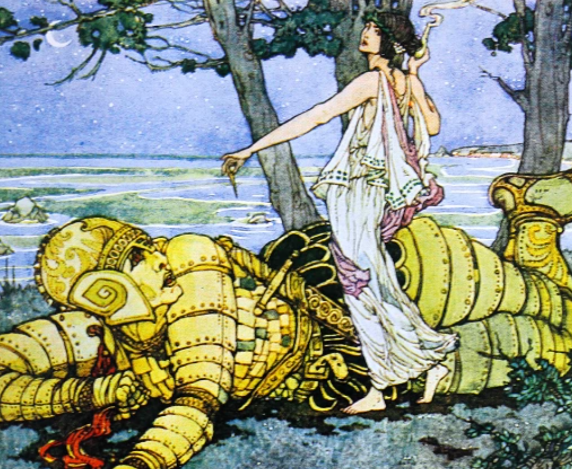
Inventors have long dreamed of creating thinking machines. Ancient Greek mythology is full of stories about inventors and artificial life, including inventors such as Pygmalion, Daedalus, and Hephaestus, and artificial beings such as Galatea, Daedalus and Talos, and Hephaestus and Pandora.

The image above is the famous painting Pygmalion and Galatea. Pygmalion was a king of Cyprus in Greek mythology. According to the Roman poet Ovid's Metamorphoses, Pygmalion was a sculptor who created an ivory statue based on his ideal image of a woman. He fell in love with his creation and named her Galatea. The goddess Aphrodite, taking pity on him, brought the statue to life.

Daedalus was the father of Icarus and the inventor of Icarus's wings. He was a famous architect and craftsman who, in addition to Icarus's wings, also built the labyrinth that imprisoned the Minotaur. Maze-solving, search, chess, path planning, and other "search" tasks were a very important part of the early development of artificial intelligence.

Sutton once said: "We must accept the bitter lesson that attempting to solve complex problems by engineering our way of thinking is not viable in the long run." Accordingly, AI can be considered to consist of two major components: learning (using data to extract patterns) and search and optimization (using computation to extract inferences).

The intelligent bronze giant Talos was invincible according to legend. In the adventure of Jason and the Argonauts to seize the Golden Fleece, the powerful sorceress Medea devised a way to defeat Talos.

In the ancient Chinese text Liezi, there is a story about Yanshi crafting an artificial human. During his travels, King Mu of Zhou encountered a man named Yanshi who had created an artificial person indistinguishable from a real human. When the artificial human flirted with King Mu's concubines, the king became furious. Yanshi, fearing for his life, disassembled the figure, revealing it to be composed of leather, wood, and other artificial materials.

When programmable computers were first conceived, people began wondering whether such machines could become intelligent—a notion that existed as early as 1842 in Lovelace's era, a full century before the first modern computer.

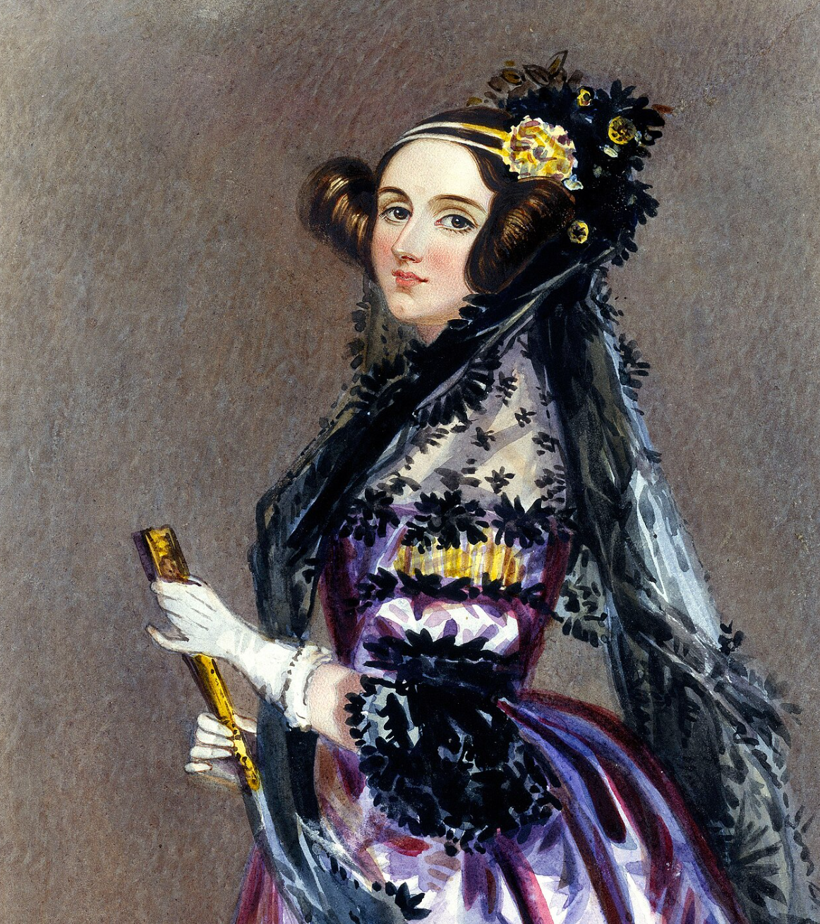
Ada Lovelace was the first person to argue that computers could be used for more than mere arithmetic, and she also published the first algorithm intended for the Analytical Engine, generally recognized as the first programmer in history. Although there is considerable debate about whether Ada was truly the first programmer, most people agree she was the first to clearly envision that the Analytical Engine could process the vast world beyond numbers. For Charles Babbage, who is posthumously honored as the father of computing and who may have written programs earlier, the Analytical Engine was simply a number-crunching machine. But Ada saw that if a machine could manipulate numbers, and numbers could represent other things—letters, musical notes, and so on—then the machine could manipulate symbols according to rules. This vision was a very early form of thinking about whether machines could become more intelligent, which is why I feel compelled to include Ada in any discussion of artificial intelligence.

Today, artificial intelligence (AI) is a vibrant field with many practical applications and active research frontiers. We use intelligent software to automate repetitive tasks, understand speech and images, perform medical diagnostics, and support fundamental scientific research.

In the early days of AI, the field quickly solved problems that were intellectually challenging for humans but relatively straightforward for computers: problems that could be described by a set of formal mathematical rules. The true challenge for AI lies in solving problems that are easy for humans to perform but difficult to formally describe—such as recognizing words in speech or faces in images. For humans, these tasks are highly intuitive, requiring almost no conscious effort, but for computers, they remained stubbornly unsolvable for a long time.

This book focuses on precisely these intuitive problems. The solution explored here is to allow computers to learn from experience and understand the world through a hierarchy of concepts, where each concept is defined by its relationship to simpler concepts. Instead of human-defined knowledge, the computer acquires knowledge through experience. This concept hierarchy enables computers to learn complex concepts by composing simpler ones. If we draw a graph showing how these concepts are built upon one another, the graph would have many layers—in other words, it is "very deep"—and hence we call this approach deep learning.

In the past, computers were often used to solve problems in idealized environments with relatively simple rules, such as chess. For humans, this is intellectually very challenging, but computers can handle it quite easily. However, things that seem trivially easy for humans—recognizing one's mother, cooking, folding blankets, sensing someone's emotions from their gestures and expressions—are extremely difficult or even impossible for computers. Thirty years ago, computers could already beat the world's best chess players, yet as of 2026 when these notes are being written, even with LLMs now capable of communicating and conversing quite well with humans, cooking and folding blankets remain tasks that robots can hardly accomplish. The real world lacks idealized environments, making it difficult for computers to express formal language. One could even say that despite how remarkably computers have developed, their essence remains what Ada envisioned two hundred years ago: operating through numbers. Even today's astonishing ChatGPT has not departed from this paradigm.

The focus of artificial intelligence development is on intelligence—a trait that humans have identified based on their own nature. What people call intelligence is essentially the mode of thinking and cognitive ability that humans themselves possess. Humans' innate ability to process elements of the real world is something computers lack. Therefore, if we want computers to learn the messy elements of the real world, only then can they potentially exhibit intelligent behavior.

In the early days of AI, knowledge bases were used to hard-code real-world knowledge into systems using formal languages. Computers could still apply logical inference rules to reason over these formal representations. However, none of these projects achieved significant success. The most famous was the 1989 Cyc project, a reasoning engine combined with a knowledge database expressed in the CycL language. Human supervisors manually entered all information—a remarkably cumbersome process. It proved extremely difficult to describe the real world accurately with sufficiently complex formal rules. For example, Cyc could not understand "there is a person named Fred who is shaving in the morning," because its reasoning engine detected a contradiction in the story: humans have no electronic components, but Fred is holding an electric razor, so the system concluded that "FredWhileShaving" was an entity containing electronic components, leading it to question: "Is Fred still a person while shaving?"

The difficulties faced by hard-coded knowledge systems demonstrated that AI systems need the ability to learn knowledge autonomously—that is, to acquire knowledge by extracting patterns from raw data. This capability is known as machine learning.

The introduction of machine learning enabled computers to tackle problems involving real-world knowledge and make seemingly subjective decisions. As noted in the first chapter of the author's reinforcement learning notes, in the 1970s and 1980s, many researchers investigating trial-and-error learning eventually transitioned to machine learning (particularly supervised learning).

Simple and common machine learning algorithms include logistic regression and naive Bayes. They can be used to identify spam email, recommend whether a cesarean section should be performed, and so on. The performance of such supervised learning algorithms depends heavily on the representation of the input data. For example, when logistic regression is used to recommend cesarean sections, it does not directly examine the patient; rather, the doctor provides the system with key information, such as whether there is a uterine scar. Each piece of information is called a feature. Logistic regression learns the relationship between these features and outcomes, but it cannot influence how these features are defined. If we give a logistic regression model an MRI image of a patient instead of a doctor's structured report, it will fail to make effective predictions, because individual pixels in an MRI image have almost no relationship to cesarean complications.

This dependence on representation is a universal phenomenon in computer science and daily life. In computer science, for instance, data retrieval operations can be greatly sped up if the data is well-structured and intelligently indexed. Humans can easily perform arithmetic with Arabic numerals but find it extremely difficult with Roman numerals. Thus, representation has a significant impact on the performance of machine learning algorithms.

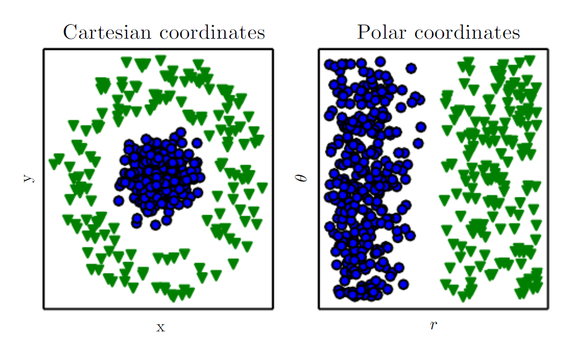
The book provides the figure above as an example: suppose we want to separate two classes of data in a scatter plot by drawing a straight line. Using the Cartesian coordinate system shown in the left panel, we cannot accomplish this task. However, if we convert the same data to the polar coordinate system shown in the right panel, drawing that line becomes very easy. Clearly, the performance of machine learning algorithms critically depends on the representation.

Many AI tasks can be solved by designing appropriate feature extraction methods and then feeding those features into a simple machine learning algorithm. For example, in speech recognition, a useful feature is an estimate of the speaker's vocal tract size, which provides clues about whether the speaker is male, female, or a child. However, for many tasks, it is very difficult or even impossible to know which features to extract. For example, if we want a program to recognize cars in images, we might think to use wheels as a feature, but wheels come in all shapes and sizes, and images may contain shadows, reflections, partial occlusions, and so on.

To address the feature extraction problem, we can use machine learning to discover not only the mapping from representation to output, but also the representation itself. This approach is called representation learning. It typically yields better performance than hand-designed representations and allows AI systems to quickly adapt to new tasks with minimal human intervention.

A representation learning algorithm can discover a good feature set for a simple task in minutes, or solve complex tasks in hours to months—tasks that would require enormous human effort to engineer features for manually.

A classic representation learning algorithm is the autoencoder. An autoencoder consists of two parts:

• Encoder: converts input data into a different representation
• Decoder: converts this new representation back into the original format

The training objective of an autoencoder is to preserve input information as much as possible—that is, encoding and then decoding should recover the original data. At the same time, it also tries to endow the new representation with certain desirable properties. Different types of autoencoders pursue different characteristics. Our goal in these tasks is typically to disentangle the "factors of variation" that explain the observed data. These factors are independent variables that influence the observations. In this context, the word "factor" simply refers to independent sources of influence; these sources are not necessarily combined through mathematical multiplication.

These factors are not necessarily quantities we directly observe; they may also be unseen objects or forces in the physical world that affect observable quantities, or simplified models or abstract concepts constructed by the human mind. For example, when analyzing speech, factors of variation might include the speaker's age, gender, accent, and the words being spoken; for car images, they might include position, color, angle, lighting, and shadows.

The reason real-world AI tasks are so difficult is largely because of this: these factors of variation simultaneously affect every data point we can observe. For example, a red car might appear nearly black in a nighttime image, and a car's outline can look very different from different angles. We typically need to disentangle these factors, retaining only the parts we care about and discarding irrelevant ones.

However, in practical tasks, extracting such high-level, abstract features from raw data is extremely difficult. When learning a representation is nearly as complex as the problem itself, representation learning seems to offer little help. This is where deep learning steps in to solve this core challenge.

Deep learning constructs hierarchical representations, expressing complex concepts through multiple layers of simpler representations. Deep learning enables computers to build up complex concepts step by step.

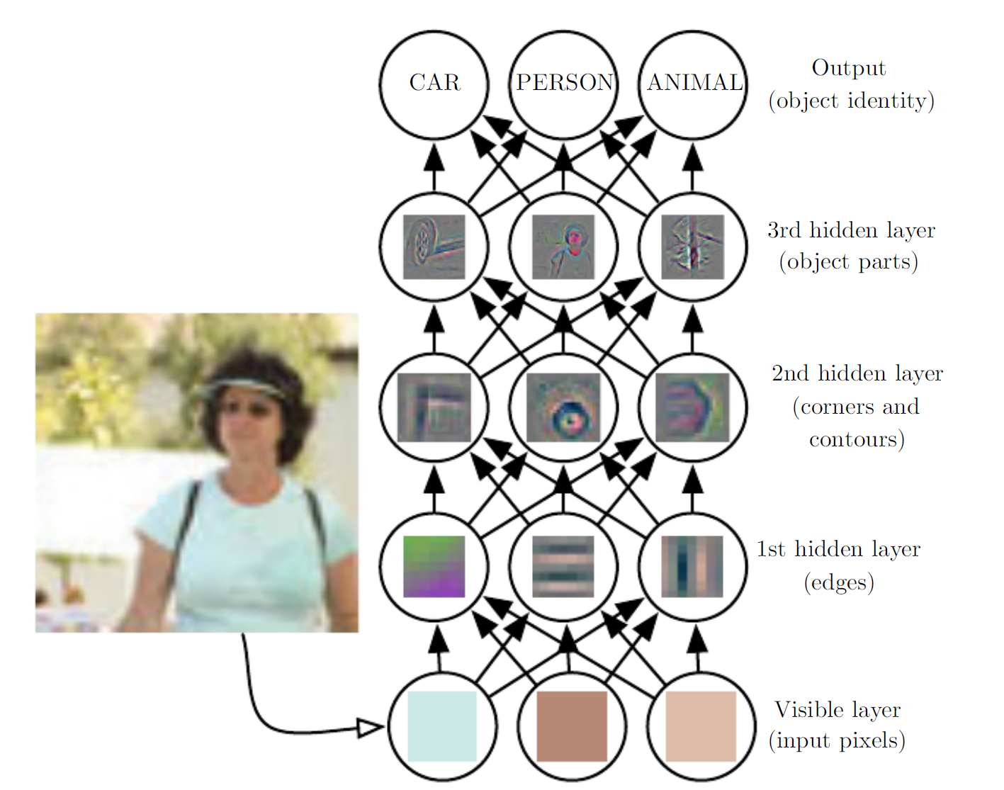
For example, as shown in the figure above, a deep learning system represents a person's image by depicting the face as a structure composed of simple shapes, such as corners and contours, which in turn are built from even more fundamental structures like edges. A computer has great difficulty understanding the meaning of raw sensory input—such an image is merely a collection of pixels to the computer, and the function mapping from a pixel set to an object's identity is extremely complex. Attempting to learn or evaluate this mapping directly seems nearly impossible. Deep learning solves this difficulty by decomposing this complex mapping into a series of nested simple mappings. Each mapping is represented by one layer of the model:

• Input is first presented at the visible layer, so named because it contains the variables we can observe.
• Then, a series of hidden layers progressively extract abstract features from the image.

These layers are called hidden because their values do not appear directly in the data; rather, the model must determine for itself which concepts are useful for explaining the observed data. The figure illustrates the types of features represented at each layer:

• The first hidden layer identifies edges by comparing the brightness of neighboring pixels.
• Building on the first layer's edges, the second hidden layer can detect corners and contours.
• Building on the second layer's contours, the third hidden layer can recognize certain parts of an object.
• Finally, through this layer-by-layer process, the model can identify the objects contained in the image.

It may appear that each layer has been "manually" assigned a specific goal, but in reality these features are learned by the model itself. Humans design the learning framework—how many layers, how many neurons per layer, whether to use convolutional or pooling layers, and so on (concepts we will learn later). The key point here is that humans only design the framework for learning; they do not define the features to be learned. Although the features at each layer may look like assigned objectives, they are actually not!

In the 1980s, neuroscientists Hubel and Wiesel discovered through their study of the visual system that human visual processing involves a series of stages, including edge detection, motion detection, stereoscopic depth perception, color detection, and so on, ultimately constructing concrete images in the brain. This discovery directly inspired the concept of "filters" in deep learning's convolutional neural networks. LeCun and others later used this principle to implement the "magical process" shown in the figure for handwritten digit recognition (LeNet), which also became the starting point for deep learning research.

A classic example of a deep learning model is the feedforward neural network, also known as the multilayer perceptron (MLP). A multilayer perceptron is a mathematical function that maps a set of input values to output values. This function is composed of several simpler functions, and we can think of each application of a different mathematical function as a new representation of the input.

There are two different perspectives for understanding deep learning:

1. The representation learning perspective: each layer learns a different representation of the input; the deeper the network, the more complex the representation; later layers can reference earlier results to form more complex logic.
2. The program execution perspective: depth allows the computer to learn a "multi-step program," where each layer is like the "memory state" after executing an operation; deeper networks can execute more instructions sequentially.

There are two main methods for measuring model depth:

1. The first view is based on the number of sequential instructions the model must execute, analogous to the longest path in a computational flow graph.
2. The second view, adopted by deep probabilistic models, considers model depth not as the depth of a computational graph, but as the depth of the graph describing how concepts are interrelated.

In some cases, the depth of the computational flow graph required to precisely compute a concept's representation may far exceed the depth of the concept hierarchy itself. For example, an AI system recognizing faces might need to iteratively reason from "whether a face is present" to determine whether another eye exists, producing a deeper computational path. Because people choose different modeling languages and graph primitives, there is no universal standard for defining model "depth." Overall, deep learning can be understood as a model construction approach that uses large numbers of learned function or concept compositions, distinguishing it from traditional machine learning.

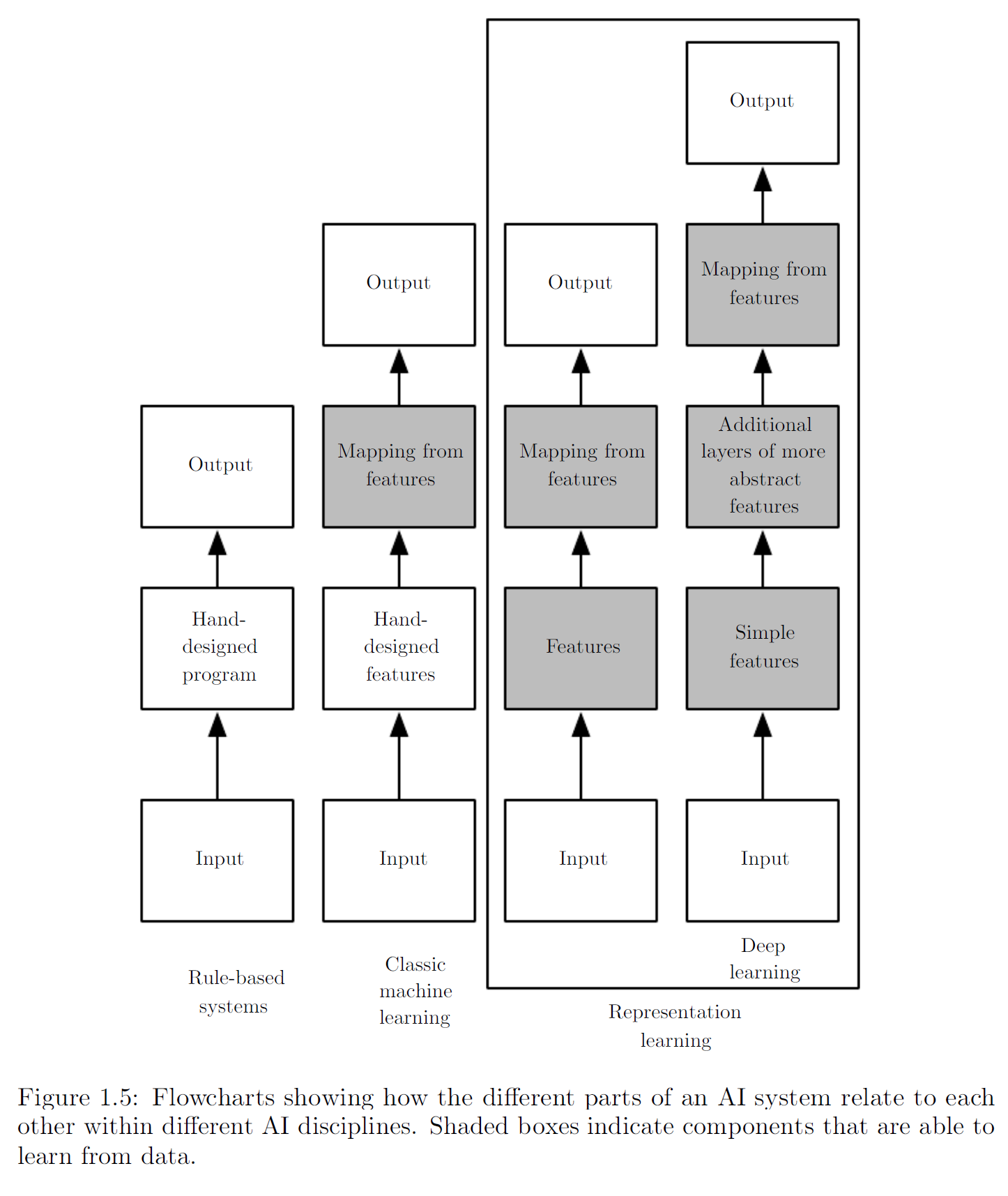
The following two figures illustrate the relationships among different AI subfields and their basic operating mechanisms.

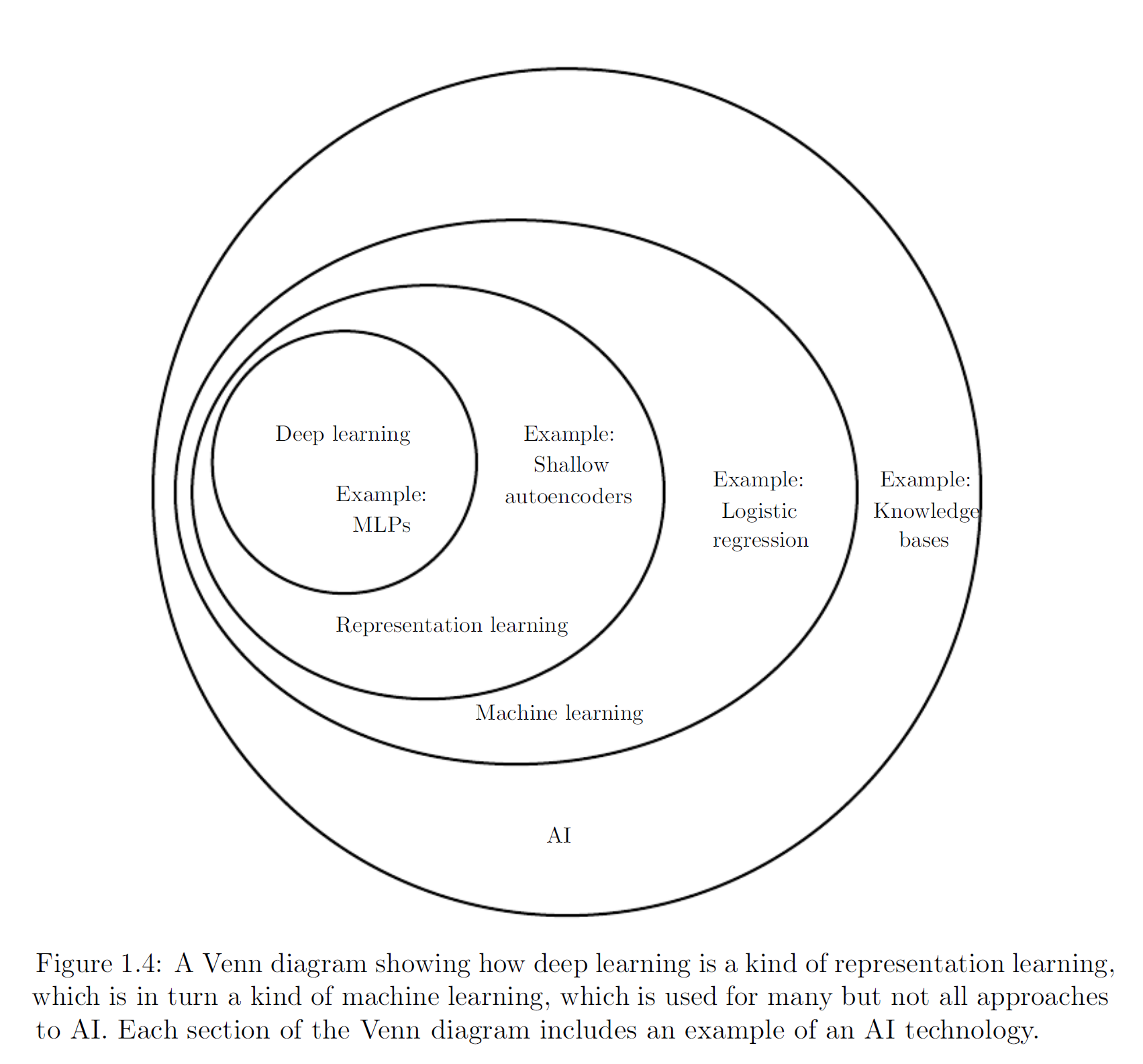
In summary, deep learning is an approach to AI and a branch of machine learning. It enables computers to continuously improve through data and experience. The author believes that in the complex real world, machine learning is currently the only viable path for building usable AI systems. What distinguishes deep learning is its ability to represent the world as a nested hierarchy of concepts: each complex concept is built upon simpler ones, and more abstract representations are derived step by step from less abstract ones.

Deep learning has been proven useful in multiple domains, including computer vision, speech and audio processing, natural language processing, robotics, biochemistry, video games, search engines, online advertising, and finance.

The First Wave: Cybernetics

Although deep learning may seem like a novel concept, its origins can be traced back to the 1940s. The field has undergone multiple renamings and was unpopular for many years before gaining traction. This section summarizes some of the basic background and development trajectory of deep learning. Overall, deep learning has experienced three waves of development:

• The first wave: the cybernetics period of the 1940s through the 1960s, during which biological theories gave rise to the earliest perceptron models capable of training a single neuron.
• The second wave: the connectionism period of the 1980s through the 1990s, characterized by the use of backpropagation to train neural networks with one or two hidden layers.
• The deep learning renaissance beginning in 2006, which only started appearing in book form around 2016.

Some of the earliest algorithms we know today were originally intended as computational models of biological learning—for example, modeling the learning process in the brain. As a result, deep learning was once called artificial neural networks (ANNs). During this period, a popular view held that the brain itself was a compelling proof that intelligent behavior was achievable, and that reverse-engineering the brain's computational principles would constitute a direct path to intelligence. At the same time, others argued that understanding the brain and the principles of human intelligence was inherently interesting and valuable, even without engineering or practical applications.

Neuroscientists discovered that mammals likely use a single algorithm to solve most of the tasks the brain handles. Particularly well-studied was the relationship between visual signals and the brain regions responsible for visual processing. Neuroscientists conducted extensive research in this direction, and "coincidences" kept emerging—people were amazed to find that certain algorithms bore a striking resemblance to neural processes within the brain.

Modern deep learning has moved beyond the neuroscience-inspired perspective on machine learning models, pointing toward a more general learning principle: multiple levels of composition. This compositional approach can be applied to various machine learning frameworks and does not necessarily require inspiration from neuroscience.

The earliest precursors to modern deep learning were simple linear models rooted in neuroscience. These models were designed to take a set of n inputs x1, ..., xn and associate them with an output y. They aimed to learn a set of weights w1, ..., wn and compute their output f(x, w) = x1w1 + ... + xnwn.

The McCulloch-Pitts neuron, proposed in 1943, was a very early model of brain function. This linear model identified two different types of inputs by checking the sign of the function \(f(x, w)\). Obviously, the weights needed to be set correctly for the output to match expectations. These weights could be set by the operator.

In the 1950s, the perceptron was the first model capable of learning weights from input samples of each category. The contemporaneous adaptive linear element (ADALINE) simply returned the value of the function \(f(x)\) itself to predict a real number, and it could also learn to predict these values from data. This simple algorithm greatly influenced the modern landscape of machine learning. The training algorithm used to adjust ADALINE's weights was a special case of what is known as stochastic gradient descent. A slightly modified version of stochastic gradient descent remains the primary training algorithm for deep learning today.

The function \(f(x, y)\) used in the perceptron and ADALINE constitutes a linear model. Linear models have many limitations—for instance, they cannot learn the XOR function, where \(f([0,1],w)=1, f([1,0],w)=1, f([1,1],w)=0, f([0,0],w)=0\): you cannot find a single straight line that separates these four points:

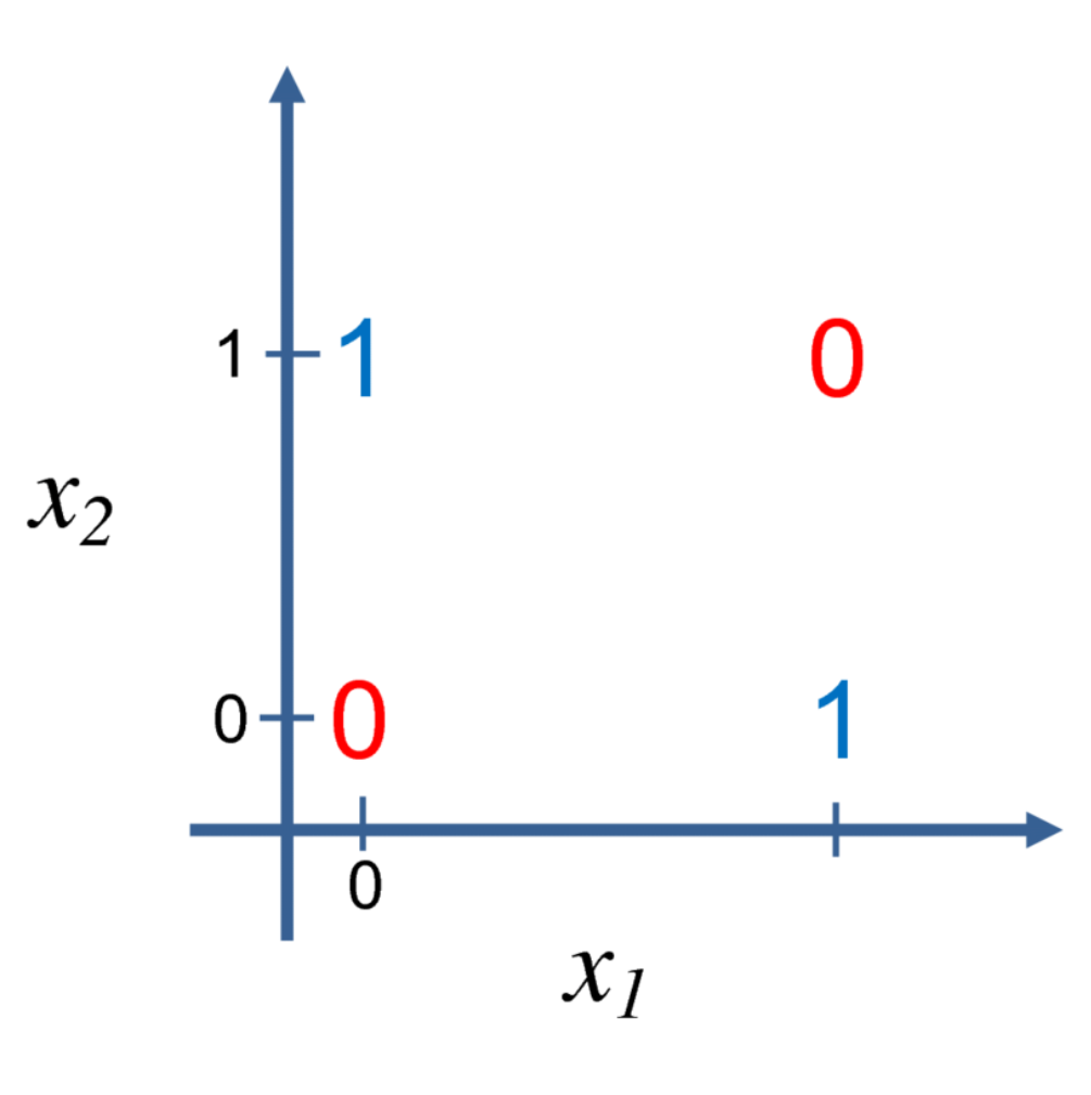
Criticism of this limitation triggered the decline of the first wave. Today, neuroscience is considered an important source of inspiration for deep learning research, but it is no longer regarded as its primary guide, because we still know very little about the brain. We do not even understand the simplest parts of the brain, let alone simultaneously monitor the activity of thousands of interconnected neurons. The direction of understanding how the brain works at the algorithmic level is now more commonly referred to as computational neuroscience. Deep learning ultimately falls within the domain of computer science, primarily concerned with building computer systems to solve tasks that require intelligence. Deep learning draws on linear algebra, probability theory, information theory, numerical optimization, and many other fields; many deep learning researchers have no interest in neuroscience whatsoever.

One of neuroscience's greatest contributions to deep learning was inspiring the idea that computational units can become intelligent through their interactions. In the 1980s, the Neocognitron, inspired by the structure of the mammalian visual system, introduced a powerful model architecture for processing images that later became the foundation for modern convolutional networks.

Most current neural networks are based on a neural unit model called the rectified linear unit. This model differs from the computational function of real neurons but can significantly improve machine learning performance.

The Second Wave: Connectionism

The second wave emerged alongside the connectionism or parallel distributed processing movement. Connectionism arose within the context of cognitive science, which is an interdisciplinary approach to understanding the mind that integrates multiple levels of analysis.

In the early 1980s, most cognitive scientists studied symbolic reasoning models, but symbolic models struggled to explain how the brain uses neurons to implement reasoning. Connectionists therefore began studying cognitive models truly grounded in neural implementation. Many of the revived ideas could be traced back to the work of psychologist Donald Hebb in the 1940s.

The central idea of connectionism is that intelligent behavior can emerge when a network connects a large number of simple computational units together. This insight applies equally to neurons in biological neural systems, which play a similar role to hidden units in computational models.

The first important concept in connectionism was distributed representation, proposed by Hinton and colleagues. The idea is that each input to the system should be represented by multiple features, and each feature should participate in the representation of multiple possible inputs. For example, if we want to recognize red, green, and blue cars, trucks, and birds, there are two intuitive approaches to representing these inputs:

• The first approach uses 3x3 = 9 possible combinations, requiring 9 neurons. Each neuron learns a specific category, such as red car, red truck, or red bird.
• The second approach uses distributed representation: three neurons for color and three neurons for car, truck, and bird. This requires only 6 neurons. Additionally, the "red" neuron can learn about redness from images of cars, trucks, and birds alike.

Another major achievement of connectionism was the backpropagation algorithm. Although it was once eclipsed, it later re-emerged as one of the dominant methods.

In the 1990s, researchers made important advances in using neural networks for sequence modeling. Hochreiter and Schmidhuber introduced Long Short-Term Memory (LSTM) networks to address these challenges. Today, LSTM is widely used in many sequence modeling tasks.

The second wave persisted until the mid-1990s. At that time, many startups based on neural networks and AI technologies began seeking investment with ambitious but somewhat unrealistic goals. When AI research failed to meet these unreasonable expectations, investors grew disillusioned. Simultaneously, other areas of machine learning, such as kernel machines and graphical models, achieved strong results on many important tasks. These two factors together led to the decline of the second wave of neural networks.

Although the second wave faded from public view, between the second wave's retreat and the third wave's rise, neural networks continued to achieve impressive results on some tasks. The Canadian Institute for Advanced Research (CIFAR) helped sustain neural network research through its Neural Computation and Adaptive Perception (NCAP) program. This program brought together machine learning research groups at the University of Toronto, the University of Montreal, and New York University, led respectively by Geoffrey Hinton, Yoshua Bengio, and Yann LeCun. This multidisciplinary CIFAR NCAP research program also included neuroscientists and experts in human and computer vision.

At that time, it was widely believed that deep networks were difficult to train. In retrospect, we now know this was because the computational cost was too high and there was no available hardware for sufficient experimentation. We now know that algorithms that existed in the 1980s could work perfectly well.

The Third Wave: Deep Networks

The third wave began with a breakthrough in 2006. Hinton demonstrated that a neural network called a deep belief network could be effectively trained using a strategy known as greedy layer-wise pre-training. Other CIFAR-affiliated research groups quickly showed that the same strategy could be applied to train many other types of deep networks and systematically improved generalization performance on test examples.

This wave of neural network research popularized the term "deep learning," emphasizing that researchers now had the ability to train deeper neural networks that were previously impossible to train, with a focus on the theoretical importance of depth. By this point, deep neural networks were outperforming competing machine learning techniques and AI systems with hand-crafted features.

At the time the book was published (2017), the third wave of deep networks was still continuing. As we have since witnessed, the introduction of the Transformer architecture and the large language models led by ChatGPT have fundamentally reshaped how people access information, and development continues at a rapid pace through 2025.

Ever-Increasing Data Volume

Many people ask: if the first experiments with artificial neural networks were conducted in the 1950s, why have they only recently been recognized as a key technology? Deep networks were long regarded as an art practiced only by experts rather than a technology. Only recently, as training data has grown, have the tricks required diminished. The learning algorithms that currently achieve human-level performance on complex tasks are nearly identical to those that struggled with toy problems in the 1980s. The key difference is the resources available for successfully training these algorithms.

Because more and more of our activities take place on computers, what we do is increasingly being recorded. Because our computers are increasingly networked together, these records become easier to centralize and organize into datasets suitable for machine learning applications. Since the primary burden of statistical estimation (observing small amounts of data to generalize to new data) has been alleviated, machine learning has become much easier in the big data era.

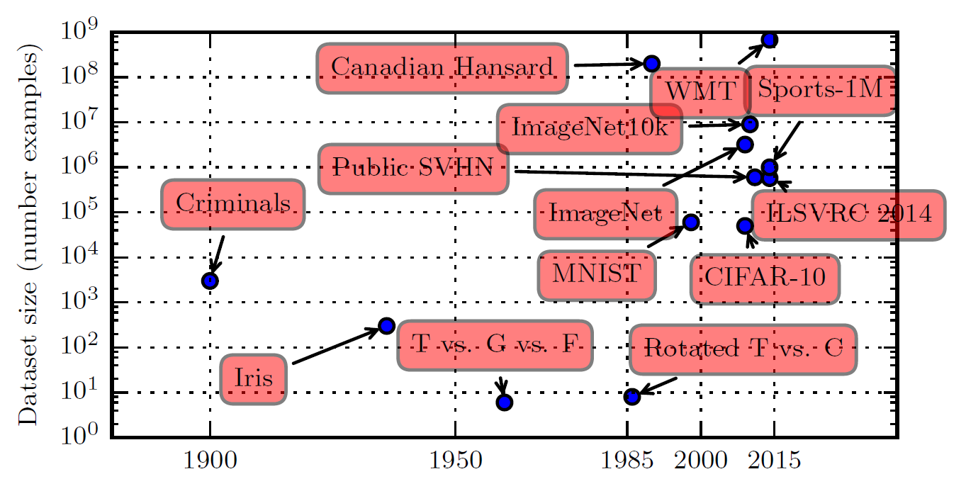
The figure above shows how benchmark dataset sizes have increased over time. A rough rule of thumb holds that supervised deep learning algorithms will generally achieve acceptable performance given approximately 5,000 labeled examples per class, and will match or exceed human performance when trained on datasets of at least 10 million labeled examples. Furthermore, achieving success on smaller datasets is an important area of research, with particular emphasis on leveraging large quantities of unlabeled examples through unsupervised or semi-supervised learning.

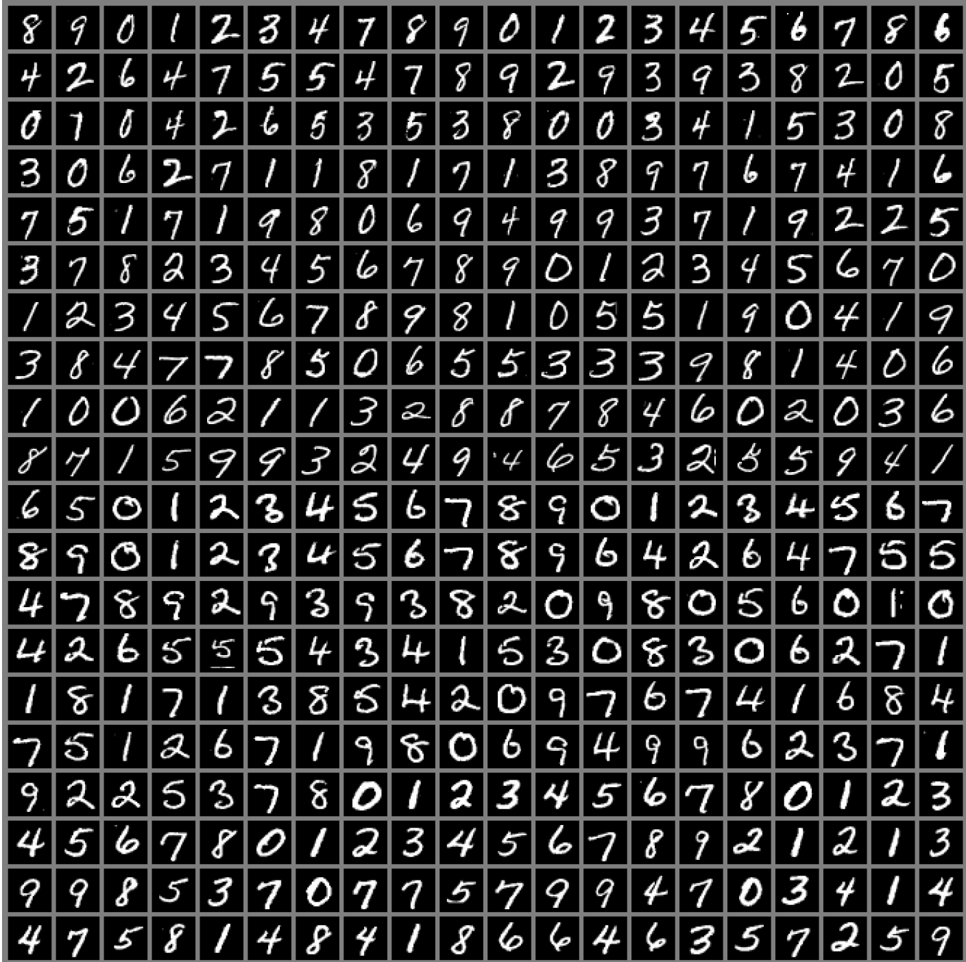
The figure above shows sample inputs from the MNIST dataset, which Hinton described as "the Drosophila of machine learning," meaning machine learning researchers can study their algorithms under controlled laboratory conditions.

Ever-Increasing Model Size

In the 1980s, neural networks achieved only modest success. Another important reason they are now so successful is that we now possess the computational resources to run much larger models. One of the key insights of connectionism is that many neurons working together become intelligent.

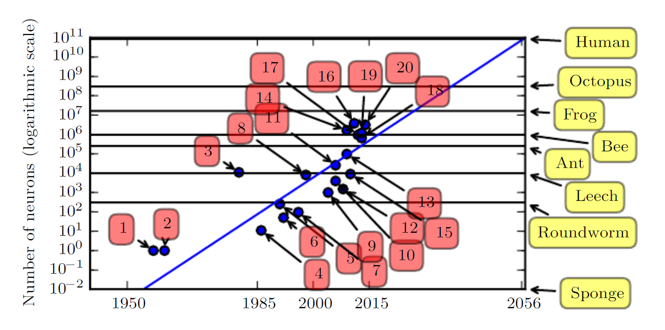
The numbers in the figure above correspond to the following models:

1. Adaptive linear element ( Widrow and Hoff, 1960 )
2. Neocognitron ( Fukushima, 1980 )
3. GPU-accelerated convolutional network ( Chellapilla et al. , 2006 )
4. Deep Boltzmann machine ( Salakhutdinov and Hinton, 2009a )
5. Unsupervised convolutional network ( Jarrett et al. , 2009 )
6. GPU-accelerated multilayer perceptron ( Ciresan et al. , 2010 )
7. Distributed autoencoder ( Le et al. , 2012 )
8. Multi-GPU convolutional network ( Krizhevsky et al. , 2012 )
9. COTS HPC unsupervised convolutional network ( Coates et al. , 2013 )
10. GoogLeNet ( Szegedy et al. , 2014a )

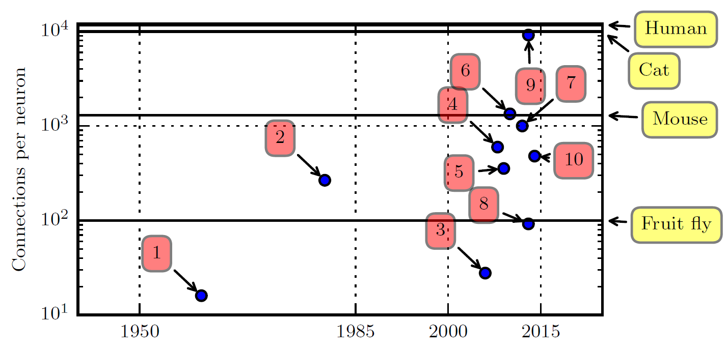
As of the book's writing in 2017, the number of neural connections in machine learning models was on the same order of magnitude as those in mammalian brains, with approximately 1,000 connections per neuron. Since the introduction of hidden units, the scale of artificial neural networks has roughly doubled every 2.4 years. This trend appears likely to continue for decades. Unless new technologies can rapidly scale up, artificial neural networks will not match the human brain's number of neurons until at least the 2050s. Biological neurons may represent functions far more complex than those represented by current artificial neurons, meaning biological neural networks may be even larger than what the figure depicts.

The numbers in the figure above correspond to the following:

1. Perceptron (Rosenblatt, 1958, 1962)
2. Adaptive linear element (Widrow and Hoff, 1960)
3. Neocognitron (Fukushima, 1980)
4. Early back-propagation network (Rumelhart et al., 1986b)
5. Recurrent neural network for speech recognition (Robinson and Fallside, 1991)
6. Multilayer perceptron for speech recognition (Bengio et al., 1991)
7. Mean field sigmoid belief network (Saul et al., 1996)
8. LeNet-5 (LeCun et al., 1998b)
9. Echo state network (Jaeger and Haas, 2004)
10. Deep belief network (Hinton et al., 2006)
11. GPU-accelerated convolutional network (Chellapilla et al., 2006)
12. Deep Boltzmann machine (Salakhutdinov and Hinton, 2009a)
13. GPU-accelerated deep belief network (Raina et al., 2009)
14. Unsupervised convolutional network (Jarrett et al., 2009)
15. GPU-accelerated multilayer perceptron (Ciresan et al., 2010)
16. OMP-1 network (Coates and Ng, 2011)
17. Distributed autoencoder (Le et al., 2012)
18. Multi-GPU convolutional network (Krizhevsky et al., 2012)
19. COTS HPC unsupervised convolutional network (Coates et al., 2013)
20. GoogLeNet (Szegedy et al., 2014a)

The data and discussion above are presented from the perspective of computational systems. In reality, however, the networks as of the timeline in the figure were no more complex than a frog's nervous system. It is therefore unsurprising that early neural networks with fewer neurons than a leech could not solve complex AI problems.

Ever-Increasing Accuracy, Complexity, and Real-World Impact

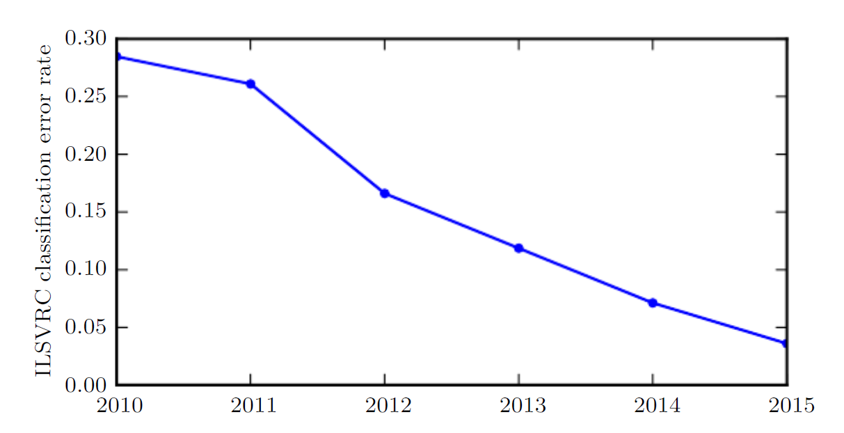
Since the 1980s, the accuracy of recognition and prediction provided by deep learning has been steadily improving. In 2012, deep learning burst onto the scene at the ImageNet Large Scale Visual Recognition Challenge, reducing the state-of-the-art top-5 error rate from 26.1% to 15.3%. Thereafter, deep convolutional networks consistently won these competitions, and by 2017, the top-5 error rate had been reduced to 3.6%, as shown in the figure below:

As deep networks have grown in scale and accuracy, the tasks they can solve have also become increasingly complex. This trend of growing complexity has been pushed to its logical conclusion with the introduction of neural Turing machines, which can learn to read from and write arbitrary content to memory cells. Such neural networks can learn simple programs from examples of desired behavior. For instance, they can learn to sort a sequence of numbers from examples of unsorted and sorted sequences. This self-programming technology is in its infancy, but in principle could be applied to virtually any task in the future.

Another of deep learning's greatest achievements is its extension into the field of reinforcement learning (RL). In reinforcement learning, an autonomous agent must learn to perform tasks through trial and error, without guidance from a human operator. DeepMind demonstrated that deep learning-based reinforcement learning systems could learn to play Atari video games and match human performance on multiple tasks. Deep learning has also significantly improved the performance of reinforcement learning for robotics.

Many deep learning applications are highly profitable. At the same time, progress in deep learning has relied heavily on advances in software infrastructure, supporting important research projects and commercial products.

Deep learning has also contributed to other sciences, such as biopharmaceuticals. The author expects deep learning to appear in an increasing number of scientific fields in the future.

In summary, deep learning is an approach to machine learning. Over the past several decades, it has extensively drawn upon our knowledge of the human brain, statistics, and applied mathematics. In recent years, thanks to more powerful computers, larger datasets, and techniques for training deeper networks, deep learning has experienced tremendous growth in both popularity and practical utility. The coming years are filled with challenges and opportunities for further advancing deep learning and bringing it to new domains.

Deep Neural Networks

A Deep Neural Network (DNN) is a broad umbrella term. Generally speaking, any artificial neural network that satisfies the following two conditions can be called a DNN:

• Composed of multiple interconnected nodes (artificial neurons)
• Has multiple hidden layers, hence the "depth"

Common deep neural networks include (in chronological order):

• MLP/DFF, deep feedforward networks, the first and most important neural network model
• RNN, recurrent neural networks, early attempts at sequence modeling
• CNN, convolutional neural networks, a major breakthrough in image recognition
• LSTM, long short-term memory networks, mature sequence modeling (an upgraded RNN)
• GAN, generative adversarial networks, which opened the era of AI generation
• Transformer, which launched the era of large models through the self-attention mechanism
• MoE, Mixture of Experts (still with Transformer at its core)
• Diffusion Models, the latest important breakthrough in the generative domain

In general, when we refer to deep learning, we mean deep neural networks.

Neural Network Architecture

The vast majority of deep neural networks are composed of structures like the following:

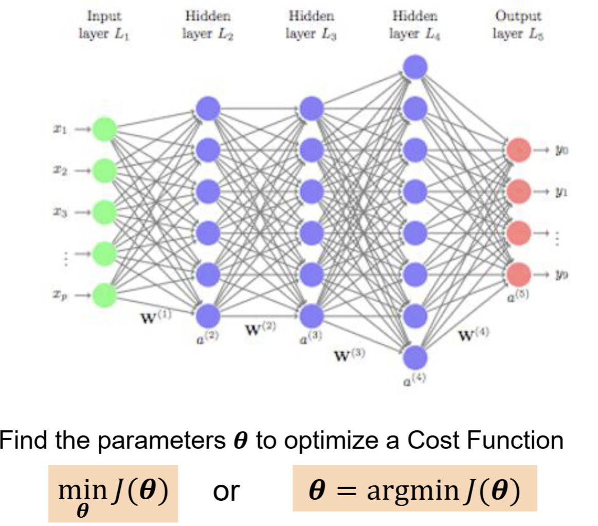
For most neural networks, our goal is to continuously adjust all internal parameters \(\Theta\) of the network so as to minimize the loss function \(J(\Theta)\), which measures how poorly the model performs. Here, the parameters are the ones between layers in the figure above, representing the transmission mechanism during neural network processing. The final result we obtain is a probabilistic conclusion, such as "80% tiger, 15% cat, 5% other."

Of course, as neural networks have evolved, different architectures have been developed for different objectives and tasks, but their core idea does not differ significantly from what is described above.

To minimize the loss function, we can imagine plotting it out. Obviously, a real neural network model cannot have only two variables, but we use single-variable and two-variable cases as analogies.

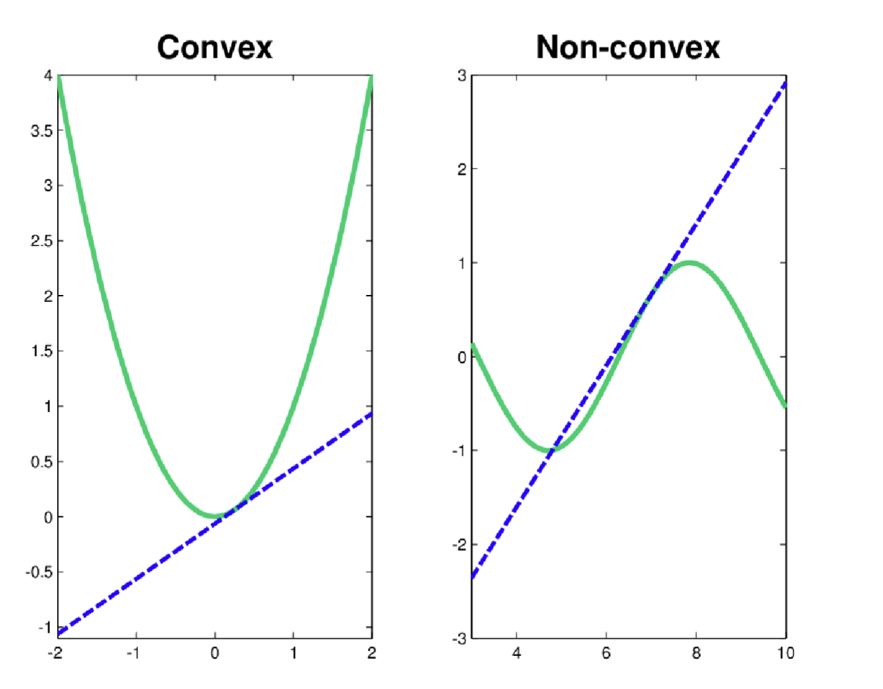
For single-variable convex and non-convex functions, the picture looks like this:

For two-variable convex and non-convex functions, the picture looks like this:

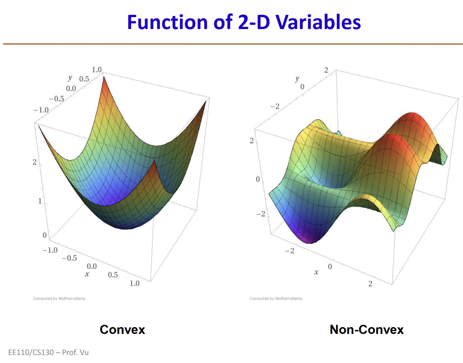
As we can see, a convex function has a single lowest point called the global optimum. A non-convex function, in addition to that lowest point, has many other "small valleys" called local optima.

The loss functions of nearly all deep neural networks are non-convex. Therefore, training a deep neural network model generally means finding the lowest point (or an approximate lowest point) of the model's loss function.

---

Now that our goal is to minimize the loss function, we need to understand what the loss function looks like. As we have seen above, a neural network is a multi-layered transmission structure. In the process of transmitting from one layer to the next, each inter-layer transition has a corresponding function. Composing all inter-layer functions together yields the neural network model itself. We use the loss function to measure the model's performance. Here are several important concepts summarized as follows:

• Input x: the vector fed into the neural network, typically high-dimensional
• \(\Theta\): all learnable parameters in the neural network, including weights w and biases b
• Neural network model: \(f(x;\Theta)\), which produces the final output given the input
• y: the ground truth label

Combining the concepts above, we obtain the Loss Function:

\[ L(f(x;\Theta),y) \]

The loss function represents the model's performance on a single example. For instance, you input an image vector and receive a result; the result indicates the image (model prediction) is a gorilla, but the image (ground truth) is actually a baboon. The deviation in the prediction is the loss. Hereafter, we will use the technical term "loss" to avoid ambiguity.

For example, suppose we encode baboon as [0,0,1,0] and gorilla as [0,1,0,0], and then feed a 100x100 pixel grayscale image into the model. The input x is a 10,000-dimensional vector. After passing through the network's layer-by-layer parameter computations, the final output is a 4-number prediction f(x;θ): [0.05, 0.1, 0.8, 0.05]. This result indicates the network thinks there is an 80% chance the image is a baboon and a 10% chance it is a gorilla. We then discover the image is actually a gorilla. Comparing [0,1,0,0] with [0.05, 0.1, 0.8, 0.05] gives us the loss.

Since we know how to compute the loss for a single image, we can compute the loss for 10,000 images. We continuously feed images into the model, compute the loss, adjust the parameters based on the loss, and ultimately reduce the loss on these 10,000 images to as low as possible. This completes one round of neural network training.

To conveniently measure this overall loss value, we need to aggregate the loss for each individual image into a unified framework. This framework is the Cost Function:

\[ J(\theta) = \mathbb{E}_{(x,y)\sim \hat{p}_{\text{data}}}\bigl[\,L\bigl(f(x;\theta),\,y\bigr)\bigr] \]

The above is an example of a cost function that uses stochastic averaging to compute the mean of all losses, yielding the overall cost. Hereafter, we use the term cost to describe the neural network model's overall loss performance across the training set.

---

Now let us take a closer look at the neural network model \(f(x;\Theta)\).

In a neural network model, after data is input, it passes through layer-by-layer computations and connections to produce a final output. For example, each node in a given layer receives inputs from the previous layer. These inputs are computed using weights W and biases b to produce a value. Every node produces such a value through this process, which we call a linear transformation:

\[ z = W^{T}h + b \]

The value z obtained at this point is an intermediate value, also called the pre-activation value.

The number of nodes, connection patterns, and parameter configurations in a neural network are determined by the model's architecture; the specific values of weights and biases are obtained through training. When each node receives the result z from the linear transformation above, it applies a nonlinear transformation to z and outputs a final signal value. This process is called activation:

\[ a = g\!\left(W^{T}x + b\right) \]

Here g is the activation function. ReLU is one such activation function. You can imagine a TV station about to broadcast a program: the production team sends the finished product to the station, and the station reviews it, finds it full of violence with potential negative impact, and blocks it from airing. This review process is analogous to activation, and blocking the broadcast corresponds to the activation function's output.

The pathway is determined by the neural network's architecture, and the value continues to be passed to the next layer through weight w and bias b computations. Through successive training iterations, weights w and biases b are continuously refined to produce a better neural network model. When we ultimately train the neural network to achieve a near-minimal cost function, the network with its trained weights and biases is our trained model.

The above outlines the general idea of neural network training. If a neural network has three hidden layers, its composite function is:

\[ f(x;\theta)=g_{3}\!\left(W_{3}\cdot g_{2}\!\left(W_{2}\cdot g_{1}\!\left(W_{1}x+b_{1}\right)+b_{2}\right)+b_{3}\right) \]

Sometimes we omit the biases b and write the neural network as:

\[ f(x;\theta)=f_{L}\circ f_{L-1}\circ \cdots \circ f_{1}(x) \]

where each layer is defined as:

\[ a^{(l)} = g^{(l)}\!\left(W^{(l)} a^{(l-1)} + b^{(l)}\right) \]

Universal Approximation Theorem

Linear models do not account for relationships among features. In image recognition, for example, pixels are not mutually independent—they influence each other. Similarly, in today's large language models, the relationship between every token in the input affects the output.

Theoretically, we could manually design a very complex function, which we call an embedding (\(\phi(x)\)). Because manually designing such a function is extremely difficult, we instead design artificial neurons:

• Input: The artificial neuron receives multiple input signals (\(x_1,x_2,...,x_n\)), similar to a biological neuron's dendrites.
• Weights: Each input signal is multiplied by a corresponding weight (\(w_1,w_2,...,w_n\)); the weight represents the importance of that input signal.
• Sum: All weighted input signals are summed to produce a total network input (Net).
• Activation Function: This aggregate Net is passed through an activation function, which introduces nonlinearity and determines whether and to what degree the neuron should be activated.
• Output: The activation function's output is the neuron's final output.

When we place multiple neurons side by side, they form a layer. All features from the input are connected to every neuron in this layer. Each neuron independently performs "weighted sum -> nonlinear activation" and produces an output. The entire process can be viewed as a parallel matrix operation (input vector times weight matrix) followed by a nonlinear transformation.

Stacking multiple such layers in series forms a deep neural network (DNN). The output of the preceding layer becomes the input to the next. Mathematically, this is a series of nested functions.

In this process, without nonlinear activation functions (nonlinearities), the entire DNN would degenerate into a simple linear function, because multiple consecutive linear transformations are equivalent to a single linear transformation. Nonlinear activation functions are therefore essential for enabling DNNs to be built deep and for each layer to learn more complex features that the previous layer cannot express.

Modern DNNs have millions or even billions of parameters (weights w). Because a DNN is a composite function, we use the chain rule from calculus to compute derivatives. The workflow is:

1. Forward propagation: starting from the input x, compute layer by layer until the final output and loss value L are obtained.
2. Backpropagation: starting from the final loss L, compute gradients layer by layer in reverse.

In practice, we do not need to implement backpropagation manually. Modern deep learning frameworks such as PyTorch, TensorFlow, and Keras have built-in automatic differentiation capabilities that automatically construct computational graphs and execute backpropagation.

Given all this effort in training DNNs, what is their theoretical advantage?

The Universal Approximation Theorem (informally stated) asserts that as long as a neural network is sufficiently wide or deep, it can approximate any continuous function f(x) to any desired precision ε:

• It can be a "shallow but wide" network (one layer with a large number of neurons).
• It can be a "deep but narrow" network (multiple layers with few neurons each).

Practice has shown that deep networks are typically more efficient than shallow ones at learning complex patterns. However, it is important to note that this theorem only guarantees that a DNN has sufficient expressive power to "represent" any function—it does not guarantee that we can find the correct weights through training (e.g., SGD) to learn that function. The learning (training) process itself is another enormous challenge.

Vanishing Gradients

Vanishing gradients occur during backpropagation, and their root cause lies in the chain rule of backpropagation. Because gradient computation in a neural network is essentially a long chain of multiplied derivatives, the gradient of the loss function L with respect to the weights W1 of the first layer can be roughly expressed as:

\[ \frac{\partial L}{\partial W_1} \approx \frac{\partial L}{\partial a_L} \cdot \frac{\partial a_L}{\partial a_{L-1}} \cdot \frac{\partial a_{L-1}}{\partial a_{L-2}} \cdot \ldots \cdot \frac{\partial a_2}{\partial a_1} \]

When most of these multiplicative terms are less than 1, their product decays exponentially as the number of layers increases, ultimately approaching zero. The main causes include:

• Saturating activation functions: for example, the derivative of the Sigmoid function has a maximum value of only 0.25, and the Tanh function's derivative has a maximum of only 1.
• Improper weight initialization: if weights are initialized to very small values, the chain multiplication also causes gradient decay.

Modern deep learning generally addresses vanishing gradients using the following methods:

• Non-saturating activation functions such as ReLU: when the input is greater than 0, ReLU's derivative is always 1, allowing gradients to flow smoothly without decay.
• Residual Connections: the core of ResNet. By creating shortcuts, gradients can skip over multiple layers and propagate forward without attenuation.
• Batch Normalization: rescales each layer's input to a distribution with zero mean and unit variance, keeping it within the "non-saturating region" of the activation function and stabilizing gradient propagation.
• Better weight initialization: using Xavier or He initialization methods to set weights at an appropriate scale from the start, maintaining stable variance in each layer's output.

Exploding Gradients

In contrast to vanishing gradients, when most of the multiplicative terms are greater than 1, their product grows exponentially with the number of layers, eventually becoming extremely large. Exploding gradients cause the training process to become highly unstable, with loss values oscillating wildly. In extreme cases, gradient values exceed the computer's representable range, causing numerical overflow and producing NaN values, which directly halt training.

The most common solutions in modern deep learning:

• Gradient Clipping: the most direct and effective approach. A maximum threshold is set for gradients; if the gradient computed during backpropagation exceeds this threshold, it is manually scaled down to the threshold value. This is like adding a volume limiter to a loudspeaker.
• Better weight initialization
• Batch Normalization

Common DNN Architectures

Each specific architecture will be covered in detail in its corresponding chapter. This section provides an overall impression.

MLP

The Deep Feedforward Network, also called a Feedforward Neural Network or Multilayer Perceptron (MLP), is a classic deep learning model. The main knowledge points for this topic are in Chapter 6 of Ian Goodfellow's classic textbook and can be studied in detail when time permits. Since we are currently progressing at a fast pace, only key points are highlighted here.

CNN

The name Convolutional Neural Networks (CNNs) comes from the mathematical convolution operation: convolution acts on two functions f and g to produce a new function. In CNNs, f is typically a filter (or kernel), and g is the image. By convolving them, a new image called a feature map is generated.

Compared to traditional fully connected networks, CNNs have unique advantages arising from two key design principles known as inductive biases:

1. Locality: The assumption that nearby regions of an image have stronger correlations. In implementation, neurons connect only to a small local region of the input image rather than to all pixels. This helps the network learn local patterns (such as edges and corners) while preserving spatial structure.
2. Translation Invariance: The assumption that a feature (such as an eye) carries the same meaning regardless of where it appears in the image. In implementation, the same filter (weight sharing) is used across the entire image to detect the same feature, meaning the network does not need to relearn how to recognize the same object at each position.

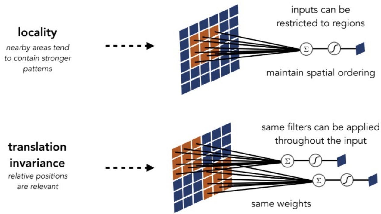
CNNs capture spatial dependencies in images through different filters. CNNs reduce feature map dimensions through pooling (or downsampling). The figure below shows the architecture and the role of each layer in LeNet (1998), a classic CNN model:

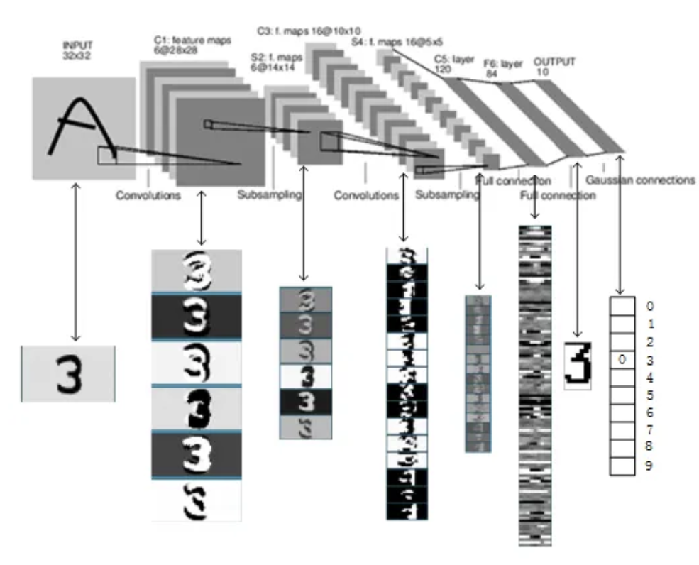
CNNs leverage two very important properties in machine learning:

1. Equivariance: \(f(g(x))=g(f(x))\)
2. Invariance: \(f(g(x))=f(x)\)

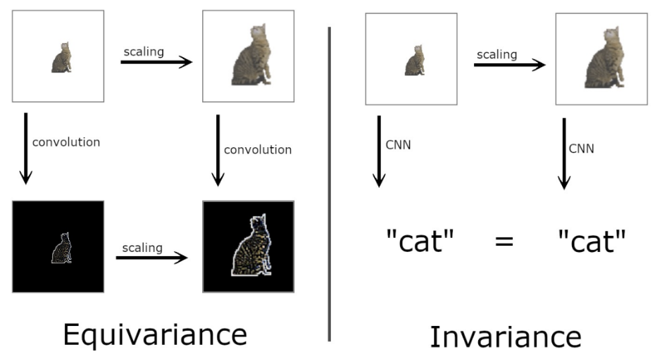
These two properties are not exclusive to CNNs, but CNNs exploit them remarkably well:

• Convolutional layers are equivariant.
• Pooling layers introduce invariance.
• The overall CNN's objective is invariant.

Furthermore, based on these properties, we can improve a model's generalization ability through data augmentation. The principle is that during training, we apply various transformations to the original data—cropping, rotation, flipping, color adjustment, and so on—artificially creating more training samples. This effectively tells the model: these images that look different all represent the same thing. By learning from these transformed data, the model learns to maintain invariance to these transformations, thereby improving generalization.

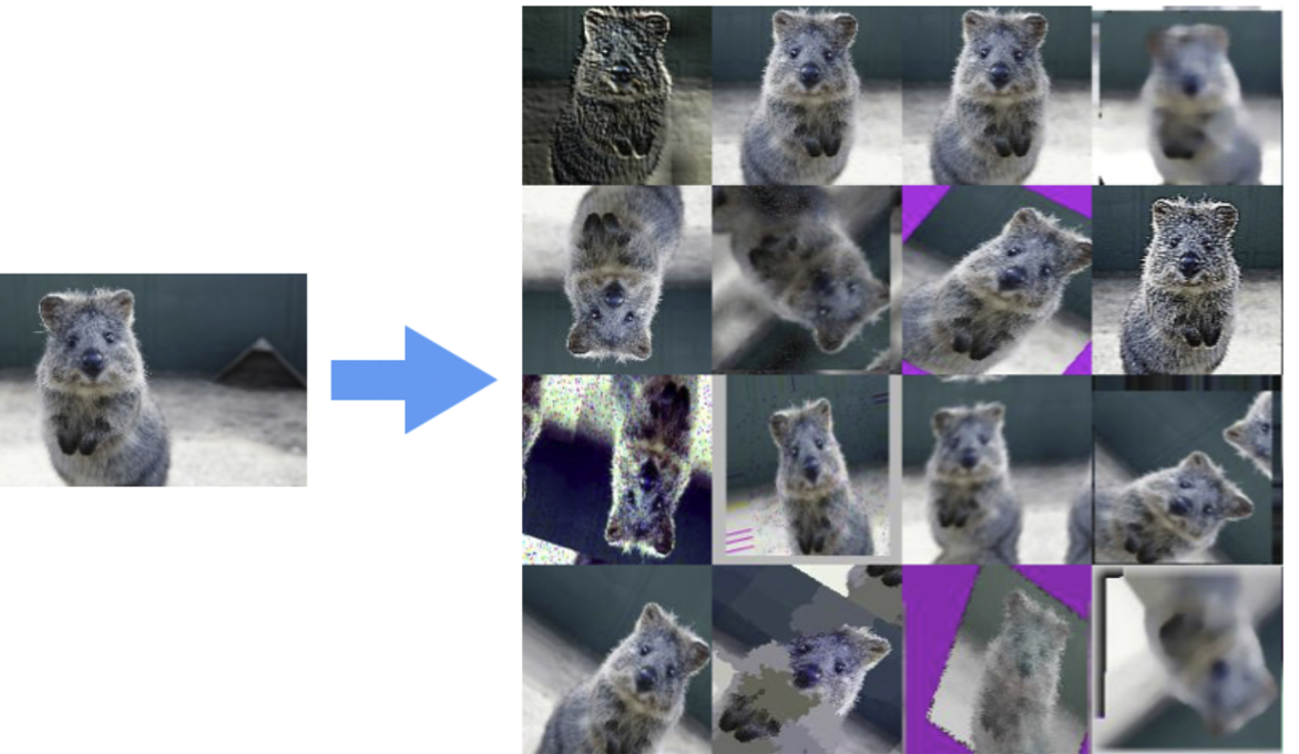
RNN

Recurrent neural networks include RNN, LSTM, GRU, and others.

Recurrent Neural Networks (RNNs) are the classic model for processing time series data. The core ideas of RNNs are:

• Sequential processing: rather than seeing all the data at once, input is read one time step at a time.
• The key is the hidden state (\(h_t\)), which combines the memory from the previous time step (\(h_{t-1}\)) with the current time step's input (\(x_t\)) to update itself, forming a new memory \(h_t\). This process is expressed as:

\[ h_t = \sigma(W_h^{T}[h_{t-1}, x_t]) \]

• The final output \(y_t\) is determined by the current time step's memory \(h_t\):

\[ \mathbf{y}_t = \sigma(\mathbf{W}_y^{\top} \mathbf{h}_t) \]

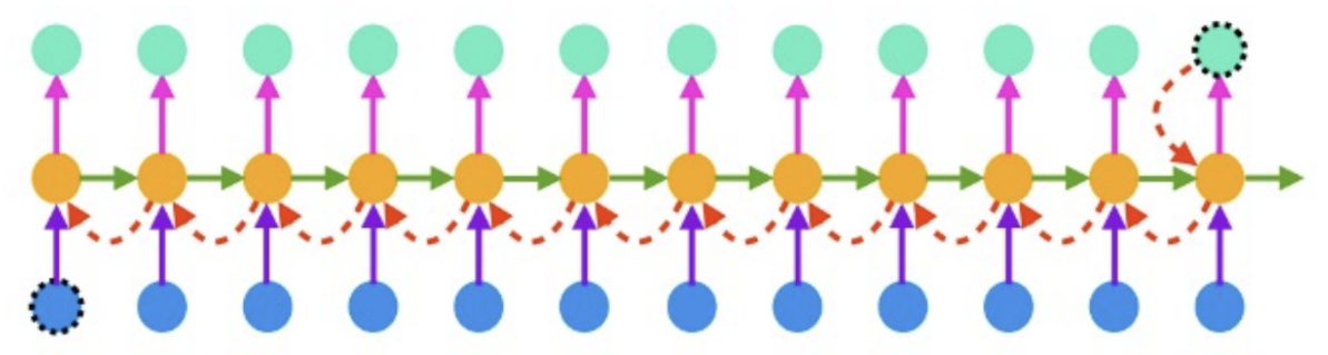
The chain structure shown above provides a very intuitive illustration of the RNN workflow:

• The bottom row of blue circles is the input layer, representing data input at different time points, forming an input sequence.
• The middle row of orange circles is the hidden layer—the core of the RNN. Each orange circle represents the hidden state at a particular time step and can be thought of as the RNN's memory up to that point, containing a summary of all previous input information.
• The hidden state \(h_t\) at time step t is computed from the previous time step's hidden state \(h_{t-1}\) and the current time step's input \(x_t\). This memory propagates forward, influencing all subsequent time steps.
• The top row of teal circles is the output layer, representing the output at each time point. The output at time step t is determined by the current hidden state \(h_t\).
• Blue upward arrows: transmit the current time step's input \(x_t\) to the hidden layer.
• Green horizontal arrows: these represent the core of the "recurrent" aspect—the transmission of memory.
• Pink upward arrows: generate output from the hidden layer's memory.
• Red backward arrows: Backpropagation Through Time (BPTT).

The core problem and fatal weakness of RNNs is difficulty in learning long-range dependencies. During training, gradients must propagate backward along this long chain (red arrows). When sequences are long, the gradient undergoes continuous multiplication during propagation, potentially leading to vanishing gradients, exploding gradients, and excessive computational and memory overhead.

---

Long Short-Term Memory (LSTM) is a very important RNN variant specifically designed to solve the standard RNN's long-term dependency problem.

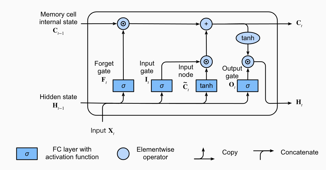
Compared to the standard RNN, which relies on a single hidden state as memory, LSTM introduces a memory mechanism capable of storing much richer information:

• A channel called the Cell State is created as the core of LSTM's long-term memory, specifically designed to store long-term information. This channel acts like a conveyor belt where information can flow easily without undergoing dramatic changes, thereby solving the vanishing gradient problem.
• Three learnable gates are created to act as managers, dynamically and selectively determining:

1. Forget Gate: Which old memories to forget? It decides how much old information to discard from the cell state; 1 means fully retain, 0 means fully discard.
2. Input Gate: Which memories to store? It decides how much new information to write into the cell state. A Sigmoid layer determines which values need updating, while a tanh layer creates a candidate new memory vector. Together they jointly update the cell state.
3. Output Gate: Which memories to output?

Through this elegant design, LSTM can actively manage information flow—retaining important long-term memories while processing current short-term inputs, hence the name "Long Short-Term Memory." Information travels along the cell state, fine-tuned only through gate control.

Generative Models

Generative models include:

• GANs are representative of adversarial generation, producing data through a game-theoretic process.
• Diffusion Models generate data by restoring from noise.
• VAEs are representative of probabilistic generation, producing data from a learned latent space.

And others.

It is important to note that while large language models (LLMs) like ChatGPT are now also being used in robotics (e.g., giving robots high-level instructions like "go to the kitchen and fetch me an apple"), the low-level trajectory generation for actually executing actions is better suited to Diffusion and similar models. Therefore, from the application perspective of robotics, introducing VAE, GAN, and Diffusion is more directly relevant. For ChatGPT-related content, see the Transformer section.

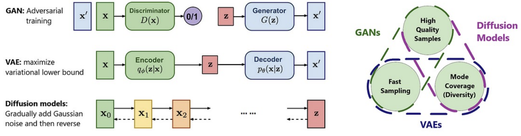
The figure above illustrates the three most popular generative model paradigms today, along with the impossible triangle:

• Quality: how realistic the generated samples are
• Speed: how fast samples are generated
• Coverage: whether the model can generate diverse types of samples, covering all modes of the real data distribution

High diversity (coverage) in the impossible triangle refers to the richness and breadth of samples the model generates. For instance, when asked to draw a dog, it should be able to produce dogs of various breeds, poses, and backgrounds. Fast sampling refers to the speed at which new samples are drawn from the model. Specifically:

• VAEs favor fast sampling and diversity (high coverage), but the quality of generated samples is typically lower.
• GANs favor generating high-quality images and fast sampling, but sometimes sacrifice diversity (mode collapse).
• Diffusion Models favor high quality and high diversity, but at the cost of very slow sampling.

Transformer

The Transformer is an entirely new architecture designed to completely replace LSTM. Its core idea is fundamentally different from RNNs. RNNs process input like a human reading—word by word—with information passing sequentially through hidden states (memory) between time steps. This structure naturally encodes sequential order information, but its drawbacks are significant: it cannot be parallelized (it must finish processing the 99th word before starting the 100th), making it very slow for long sequences. Moreover, RNNs have clear problems with long-range dependencies. LSTM alleviates this issue, but information from the first word to the hundredth still has to pass through 99 steps—too long a path, and information may still be lost.

The Transformer completely abandons the RNN paradigm, instead adopting a Self-Attention mechanism: it sees the entire sentence at once and computes the importance or relevance of every word to every other word. Its processing mechanism is parallel—all words' importance scores are computed simultaneously—thus taking full advantage of modern GPUs' parallel computing capabilities. At the same time, the distance between any two words in the sentence is always 1, so the model can directly establish a connection between the first word and the hundredth word without information having to propagate step by step.

Some critically important core concepts in the Transformer:

• Positional Encoding: Because the Transformer sees all words at once, it inherently cannot distinguish "dog bites man" from "man bites dog." Therefore, the Transformer assigns each word a unique numerical vector as a positional encoding to record its position in the sequence.
• Encoder: Receives and fully reads the input information, then compresses it into a set of information-rich numerical vectors (called context vectors or memory). Encoding strips language away from the words themselves, converting it into vectors representing concepts. The process of converting human language into numerical vectors is encoding.
• Decoder: Receives the concept vectors from the Encoder, then generates the target output word by word based on the abstract meaning these concept vectors represent. The process of converting numerical vectors into concrete human language is decoding.

Note that positional encoding is a concept unique to the Transformer, while the Encoder and Decoder were proposed earlier in the Seq2Seq (Sequence-to-Sequence) architecture. The Transformer's revolutionary contribution was implementing the Encoder and Decoder in an entirely new way. In RNNs, the Encoder and Decoder each consist of an RNN; the same applies to LSTMs.

---

In deep learning, embedding is a process that converts discrete, non-numerical categorical data (such as words, user IDs, movie names) into continuous, dense, low-dimensional numerical vectors. The result (the converted numerical vector itself) is also called an embedding or embedding vector.

For example, if the dictionary contains 50,000 words, you could create a 50,000-dimensional vector. For the word "cat" (assuming it is the 500th word), you set position 500 to 1 and everything else to 0. However, this approach yields excessively high-dimensional, very sparse vectors. All word vectors are mutually independent (orthogonal), unable to capture relationships between words. For instance, the relationship between "cat" and "kitten" looks mathematically identical to that between "cat" and "car."

A better embedding approach: instead of a 50,000-dimensional vector, we use a dense vector of, say, 300 dimensions to represent "cat":

• "cat" -> [0.12, -0.45, 0.98, ..., 0.67] (a 300-dimensional floating-point vector)

This vector is not random—it is learned by training a neural network on large amounts of data. The network adjusts the values in the vector so that words with similar meanings have vectors that are close together in multidimensional space. A classic example: embedding("king") - embedding("man") + embedding("woman") is very close to embedding("queen") in vector space. embedding("kitten") and embedding("cat") will have very similar vectors.

In summary, an embedding is a learnable lookup table. Given a word (or ID) as input, it outputs a low-dimensional dense vector representing its semantic information, which serves as the actual input for subsequent neural network layers.

In the Transformer, embeddings are taken to their extreme, with one key addition: positional encoding. Let us walk through the specific steps a Transformer takes to translate an English sentence into French, to see how the Transformer proceeds step by step:

Phase 1: Encoder

Phase 1, Step 1: Understanding the Input Sentence

1. Tokenization: Split the sentence into minimal units (tokens). Suppose we input the sentence "The cat sat." First, we tokenize it into: "The", "cat", "sat".
2. Token Embedding: Each token is converted through a learnable embedding layer (lookup table) into a fixed-dimensional numerical vector. For example, if the vector dimension is 512, the sentence becomes 3 vectors of 512 dimensions each.
3. Positional Encoding: Before feeding the word vectors into the model's main body, a positional encoding vector is added to each word vector. Thus, the final input = Token Embedding + Positional Encoding, so each vector the model receives simultaneously contains the word's semantic information (from the token embedding) and positional information (from the positional encoding).

Phase 1, Step 2: Encoder Layer Processing

These prepared vectors are fed into a structure consisting of N stacked identical encoder layers (N=6 in the original paper). Here is how one layer works:

1. Multi-Head Self-Attention: This mechanism allows every word in the sentence to "see" all other words, enabling contextual understanding. For the word "cat," self-attention computes importance scores for "The" and "sat" in understanding "cat." It then performs a weighted sum of all word vectors based on these scores, generating a brand-new "cat" vector enriched with the entire sentence's contextual information. This process occurs simultaneously for all words in parallel. "Multi-head" means this process is performed in parallel multiple times (e.g., 8 times), each focusing on different aspects (e.g., one head for syntactic relationships, another for semantic relationships). All heads' results are concatenated for richer information.
2. Add & Norm: Residual Connection and Layer Normalization: The self-attention layer's input is added directly to its output (this is called a residual connection), followed by layer normalization. This technique helps networks train more stably and go deeper.
3. Feed-Forward Network: The output from the previous step is independently passed through a simple fully connected neural network. This increases the model's nonlinear capacity for further information processing.
4. Add & Norm again.

Steps 4-7 constitute a complete encoder layer. The 6 encoder layers process the vectors sequentially, with each layer making the vector representations richer and more abstract. At the end of the encoding phase, we obtain a set of final vectors (one per input word) that represent the encoder's "deep understanding" of the original sentence, available for the decoder to consult at any time.

Phase 2: Decoder - "Generating" the Output Sentence

The decoder's goal is to use the "understanding" provided by the encoder to generate the French translation word by word. This is an auto-regressive process.

First, the decoder receives a special start-of-sequence token as its initial input, signaling it to begin generation. The decoder is likewise composed of N=6 stacked decoder layers. Here is how one layer generates the first French word:

1. As with the encoder, the start token undergoes word embedding and positional encoding.
2. Masked Multi-Head Self-Attention: Self-attention with a mask ensures the decoder can only "see" words it has already generated when producing the current word. The process is similar to the encoder's self-attention, but with a "mask." Since only the first word is being generated, it can only see the start token <s>. The mask prevents the model from "cheating" by peeking at future answers.
3. Cross-Attention: This is the bridge connecting the encoder and decoder, allowing the decoder to review the encoder's understanding of the original English sentence. This layer's input comes from the previous step (masked self-attention), but its computation queries the encoder's final output vectors. It asks: "Given that I need to generate a French word now, which words in the English sentence are most important?" It might find that "The" and "cat" are most relevant at this moment.
4. Feed-forward network and normalization: identical to the steps in the encoder (residual connection, layer normalization, feed-forward network...).

Output Embedding: At the end of the Decoder, the model generates a final vector. To convert this vector back into a specific word, it passes through a linear layer and a Softmax layer. This linear layer is essentially an embedding layer (often sharing weights with the input Token Embedding), projecting the high-dimensional semantic representation back into the vocabulary space to predict the most likely next word.

To illustrate with our translation task: after processing through N=6 decoder layers, we obtain a final output vector. This vector passes through a Linear Layer that expands its dimensionality to the entire French vocabulary size (e.g., 30,000 words). Then a Softmax function converts these values into generation probabilities for each word. We select the word with the highest probability, say "Le", as the first output.

"Le" now becomes the decoder's new input at the next time step. The decoder then repeats the entire process until it generates a special end-of-sequence token </s>:

1. Prepare the new round of input. The input sequence is now <s> and "Le". These two words undergo word embedding and positional encoding respectively, forming a new input sequence vector.
2. Pass through the decoder layers again: this new sequence vector is fed into the N=6 decoder layers. In the Masked Multi-Head Self-Attention step, the model processes <s> and "Le". When computing attention for "Le", the mask ensures it can only attend to itself and the preceding <s>, not future tokens. In the Cross-Attention step, the decoder again reviews the encoder's understanding of "The cat sat." But this time, the question becomes: "I've already said 'Le'—what word should I generate now?" The attention mechanism may now focus heavily on the encoder output vector corresponding to "cat."
3. Subsequent feed-forward network steps are identical to before.
4. Generate the second word: After all decoder layers, the final output vector passes through the linear layer and Softmax function, predicting the next most likely word—this time probably "chat".
5. Repeat: "chat" is appended to the end of the input sequence. In the third round, the decoder's input is <s>, "Le", "chat". It repeats all the above steps, using cross-attention to focus on "sat" in the English sentence, and ultimately generates "s'assit".

This auto-regressive process continues, with each step using the previous step's output as input for the next, until the model predicts that the highest-probability word is the special end-of-sequence token </s>. When this token is generated, the decoding process stops and the translation task is complete.

Ultimately, through this word-by-word, iterative generation process, the model translates "The cat sat" into "Le chat s'assit."

---

The Transformer is an extremely versatile architecture whose influence has extended far beyond its original domain of natural language processing (NLP). Some of today's most famous large language models, such as GPTs (Generative Pre-trained Transformers), PaLM, and LLaMA, are all built on the Transformer architecture without exception.

The Transformer has also been applied to computer vision: the Vision Transformer (ViT). ViT divides an image into small patches, then "flattens" these patches into a sequence. ViT then processes this patch sequence using a standard Transformer Encoder, just as it would process words in a sentence, thereby accomplishing tasks like image recognition. This completely upended the computer vision field that was previously dominated by CNNs.

In reinforcement learning, the Decision Transformer solves RL problems through sequence modeling: it treats RL trajectories (a series of "state-action-reward" tuples) as a long sequence. It then trains a Transformer model to predict the next "action" in this sequence. This transforms a complex decision-making problem into a sequence prediction problem at which Transformers excel.

The Transformer's success is no accident—it is highly scalable: thanks to its parallelized design (free from RNN's sequential dependencies), we can consistently and significantly improve performance by increasing model size, data volume, and computational resources. The current large language model race is essentially a direct manifestation of the Transformer architecture's scalability.

Transformer vs. Traditional Models:

• vs. CNN: CNN's "field of view" is limited by the kernel size, making it difficult to capture global and long-range dependencies.
• vs. RNN/LSTM: RNN/LSTM must process data sequentially, resulting in slow training speeds, and despite mitigation efforts, learning long-range dependencies remains difficult due to vanishing gradients.
• vs. MLP (Fully Connected Networks): Excessive parameter counts and inability to handle variable-length inputs (such as sentences of different lengths).

In Sutton's famous essay The Bitter Lesson, he bluntly states that AI's most painful lesson is that methods attempting to replicate human knowledge and build intricate rules have always lost in the long run to methods that are simple, general, and able to fully leverage massive computation. The two winning general methods are Search and Learning. The Transformer is the perfect exemplar of the "Learning" approach. Its simple, general design enables it to maximize the use of today's massive data and computing power, achieving astonishing intelligence through "brute force" learning.

It is worth noting that although we all know ChatGPT and other modern generative large language models are built on the Transformer architecture, the Transformer itself is an architecture, not a model type. Strictly speaking, ChatGPT belongs to a major class of generative models different from VAE, GAN, and Diffusion (covered in the following sections)—namely, Autoregressive Models.

The Transformer can be used for both generative and discriminative models:

• GPT, decoder-only. GPT's sole task is to predict the next word in a sequence, making it a purely generative model. Typical applications: chatbots, essay writing, code generation.
• BERT, encoder-only. BERT's goal is deep text understanding; its core tasks involve understanding and classifying data. Typical applications include sentiment analysis, text classification, and question-answering systems.

---

评论