Optimization Theory

Optimization Theory is a branch of mathematics that studies "how to find the best solution among all possible solutions." In the context of computer science and machine learning, it investigates how to find a set of parameters \(\theta\) that maximizes or minimizes an objective function \(f(\theta)\) (typically a loss function).

The goal of deep learning is for models to perform well on unseen data, so the "optimization objective" in deep learning carries an additional generalization requirement compared to classical optimization theory. For this reason, I have placed optimization and regularization together in this notebook. The specific rationale can be found in the "Risk Function and Empirical Risk Function" section below.

Numerical Computation in Computers

For more on numerical computation, see the Mathematics / Numerical Computation notes.

Numerical Solutions

The optimization process in deep learning is essentially a search for a set of neural network parameters that minimizes the loss function. This process relies almost entirely on numerical methods, especially gradient-based iterative optimization algorithms. Specifically, a typical neural network training optimization process proceeds as follows:

1. Forward propagation: Input data passes through the network to produce a prediction. This involves extensive matrix multiplications and activation function evaluations — pure numerical computation.
2. Loss computation: A loss function measures the discrepancy between the predicted and true values — again, numerical computation.
3. Backpropagation: To adjust parameters and reduce the loss, we compute the gradient (partial derivative) of the loss function with respect to every parameter. The commonly used backpropagation algorithm is itself a numerical method.
4. Parameter update: An optimization algorithm such as Adam uses the computed gradients to fine-tune all parameters in the network. This is a repeatedly iterated numerical approximation process.

The specific procedures listed above will be covered in subsequent sections. The reason for mentioning them here is to emphasize that numerical computation is at the core of machine learning and deep learning — mastering it is a prerequisite for everything that follows.

The vast majority of machine learning problems (e.g., training a complex neural network) are so complex that there is simply no closed-form formula that directly yields the optimal parameters. In other words, machine learning algorithms must rely on an iterative process to progressively refine their solution estimates, rather than deriving a solution through an analytical approach.

Common application scenarios of numerical computation:

• Optimization: finding a set of parameters that minimizes the loss function in deep learning
• Solving systems of linear equations: encountered, for example, in classical linear regression models

Overflow and Underflow

We have established that numerical computation is the core of machine learning and deep learning. Ideally, through thousands of iterations, the parameters would smoothly and steadily converge toward the minimum of the loss function. However, this mathematically perfect process cannot be perfectly realized on a computer. The foremost obstacle is overflow and underflow:

• Overflow: When a number is too large and exceeds the maximum representable range of the computer, it becomes infinity (inf) or a meaningless value (NaN, Not a Number).
• Underflow: When a number becomes too close to zero — beyond the minimum precision the computer can represent — it gets "rounded" to zero.

For example (do not worry about the specifics of the methods yet — this is just to build intuition about overflow and underflow):

• During backpropagation, the gradient computation involves a chain of multiplied derivatives. If the network is deep and the activation function's derivative is consistently less than 1, the gradient shrinks exponentially as it propagates backward, eventually becoming so close to zero that the computer treats it as zero.
• Conversely, if the gradient is consistently greater than 1 during backpropagation, the chain product grows enormously, exceeding the computer's maximum representable value, and ultimately becomes inf or NaN. Once a NaN appears in any update step, the entire model is instantly destroyed and training fails.

One might ask: Python already supports arbitrary-precision integers, so why not simply support 100,000 decimal places and convert everything to integers? In theory this is possible, but the computational efficiency would be abysmal. A reasonably sized deep learning training run involves trillions of computations, so numerical computation speed is critically important.

The standard modern approach is to embed circuits that natively support 32-bit and 64-bit floating-point arithmetic directly on the chip. These small units are called FPUs (Floating-Point Units). They can complete a floating-point addition or multiplication in a single clock cycle — extremely fast. Think of an FPU as a chef who does one thing: floating-point arithmetic (addition, subtraction, multiplication, division), and does it blazingly fast as a physically real entity. A single GPU contains thousands of such "chefs," coordinated efficiently through the CUDA architecture.

The physical limitations of FPUs are obvious: overflow and underflow are prominent issues. For example, if the input vector in a computation is: \(x=[1000,990,980]\)

Our FPU uses the float32 standard, which can represent a maximum value of \(3.4 \times 10^{38}\). Any computation exceeding this causes the FPU to report overflow and return inf.

Here, let us not discuss why the following formula is used — this is just to illustrate what to do in an overflow scenario:

\[ \mathrm{softmax}(\mathbf{x})_i = \frac{\exp(x_i)}{\sum_{j=1}^n \exp(x_j)}. \]

The very first step already exceeds the FPU's limits — the first computation yields no valid result. The program continues to compute \(e^{990}\), \(e^{980}\), all returning inf, and the entire computation collapses. We cannot obtain the desired result.

To solve this, we must adjust the input vector \(x\) in some way. As long as we can shift the values so that the computation does not overflow, we are fine. This kind of adjustment is generally called "numerical stabilization."

Using the same vector \(x\) as an example, here is one numerical stabilization method:

1. Find the maximum value in vector \(x\): max(\(x\)) = 1000
2. Subtract this maximum from every element, yielding a new vector \(z=[0,-10,-20]\)
3. Compute the softmax on the new vector — this transformation does not change the final softmax probabilities (because the relative contributions remain the same)
4. Thanks to the clever choice of max(\(x\)), the denominator always contains at least one \(\exp(0)=1\), and any underflowed terms are simply treated as 0. This way, the softmax result can always be computed without error. In other words, the overflow problem is solved, and underflow turns out to be harmless in the softmax computation, so it does not cause computational failure.

Of course, modern deep learning frameworks such as PyTorch and TensorFlow have already encapsulated these numerical computation procedures, so users do not encounter overflow or underflow issues. For example, when calling torch.nn.functional.softmax, the numerical stabilization method described above (and in fact even more sophisticated stabilization techniques!) is already built into the function — we simply call it directly.

Ill-Conditioning

Ill-conditioning means that for a given function, a tiny change in the input can significantly affect the output. Ill-conditioning is a major problem in numerical computation on computers because computers always introduce small rounding errors when storing numbers — for instance, storing 1/3 as 0.3333333. When such a small, unavoidable error lands on an ill-conditioned input, the output can deviate enormously from the true value.

Since one of the core tasks in deep learning is optimization — finding a parameter set that minimizes the loss function — we can visualize the loss function as a very complex, uneven terrain surface. Our goal is to reach the lowest point of this terrain. In deep learning, this terrain is often ill-conditioned: it is not smooth but rather resembles a canyon, extremely steep in some places and extremely flat in others, as shown below:

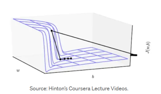
This ill-conditioned loss surface has the following characteristics:

• Steep cliffs where the loss function changes very rapidly in certain directions
• Flat valleys where the loss function changes very slowly in certain directions

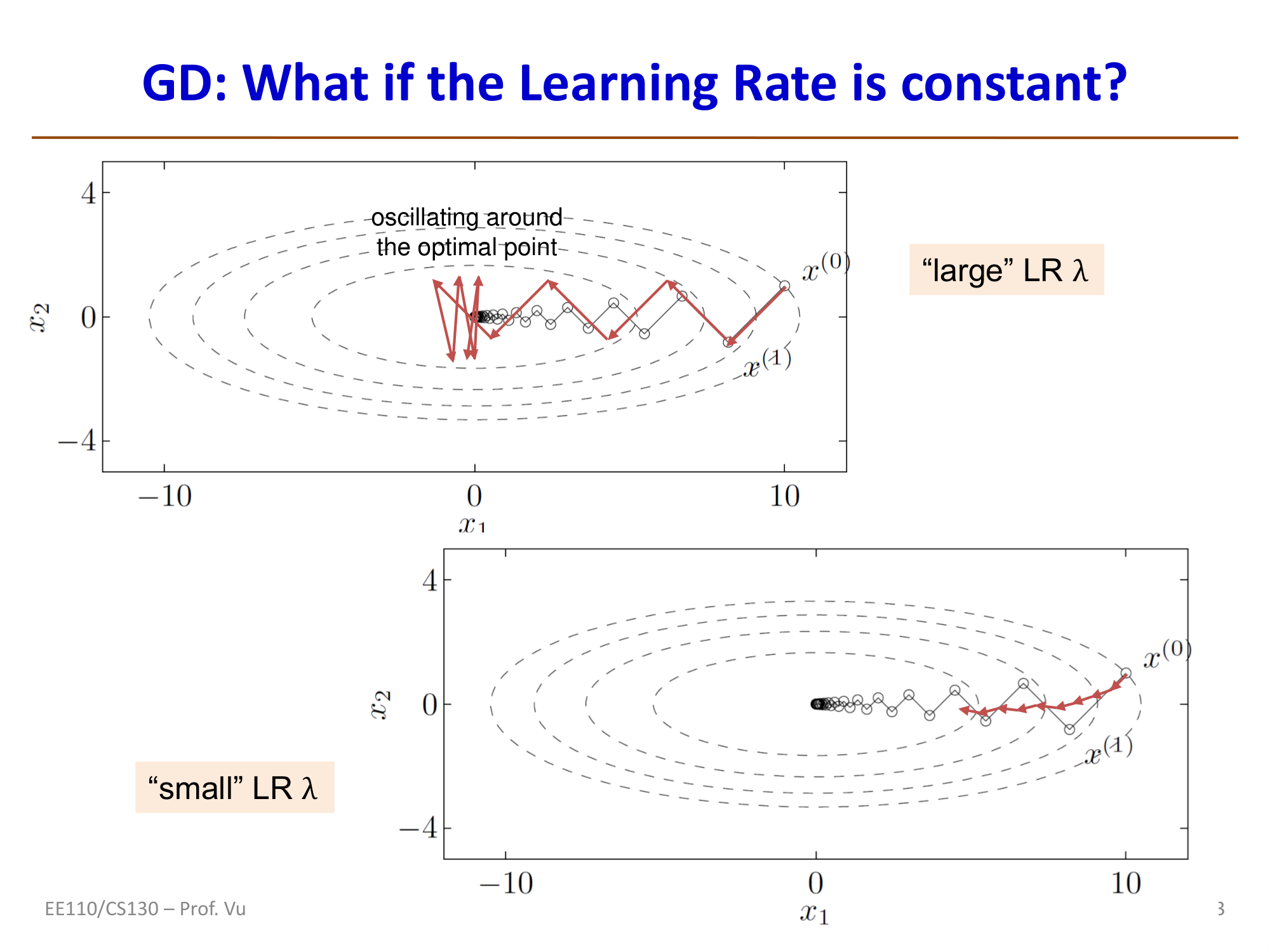
These characteristics cause our optimization algorithm (e.g., gradient descent) to encounter trouble when entering such a canyon: the gradient is very large in the steep direction and very small in the flat direction, causing the optimization process to oscillate back and forth across the canyon walls rather than progressing toward the true minimum. To prevent oscillation, we must use a very small learning rate, but this in turn makes progress in the flat direction extremely slow, potentially causing training to stall or fail to converge.

Note that the 3D plot above is merely an analogy. The loss function of a real neural network has parameters forming a very high-dimensional vector — far beyond three dimensions. Even a medium-sized model may have millions (million-dimensional) or even billions (billion-dimensional) of parameters. The 3D canyon plots used here and in most textbooks are for intuitive understanding — a dimensionality-reduced visual analogy. In other words, any 3D visualization, however constructed, is an extreme simplification — a heavily distorted slice — but sufficient for understanding important concepts such as ill-conditioning (canyons), local minima (small pits), and so forth.

Now that we understand these characteristics of ill-conditioned loss surfaces, we can adopt a targeted strategy:

• When in a flat valley, move forward at a faster pace
• When on a steep cliff, move more slowly

This strategy is, in essence, the core idea behind modern optimizers. Note that not every optimizer possesses this capability: traditional GD (Gradient Descent) and SGD (Stochastic Gradient Descent) lack this dynamic adaptivity, while Adam and SGD with Polyak momentum do have it. This capability generally consists of momentum and adaptive learning rate, which we will discuss in detail later. Before studying advanced optimizers with dynamic capabilities, we must start from the most traditional optimizers and understand basic concepts such as gradient descent.

Optimization in Deep Learning

Risk Function f and Empirical Risk Function g

In deep learning, our ultimate goal is for the model to perform well on unseen data. What we truly want to find is the expected risk (or true risk), whose mathematical formula is:

\[ f(w) = E_{(x,y) \sim P}[l(w; x, y)] \]

where:

• \(w\) represents the weight parameters of the current deep learning model.
• \(l(w; x, y)\) is the loss function for a single sample. It measures how large the error is between the model's prediction for input \(x\) and the true label \(y\), given parameters \(w\).
• \(P\) represents the complete probability distribution of data in the real world. It encompasses all possible inputs and outputs in existence.
• \(E\) denotes expectation, which can be understood as a weighted average.

The risk function \(f\) evaluates: if you were to apply your current model to all possible data from the real world, how large would the average error be? It is the most perfect standard for evaluating a model's true capability (i.e., the absolute measure of generalization ability).

We can never obtain the true distribution \(P\). For instance, in face recognition, it is impossible to collect photos of every human face under every lighting condition and every angle. Since we cannot access all inputs and outputs, we simply cannot compute the exact value of \(f(w)\) on a computer.

---

We define another function — the empirical risk — to represent model performance measured on the training set. Its mathematical formula is:

\[ g(w) = \frac{1}{n} \sum_{i=1}^n l(w; x_i, y_i) \]

where:

• \(n\) is the total number of training samples you actually have.
• \(x_i, y_i\) is the \(i\)-th specific data sample and its true label that you have collected.
• \(\Sigma\) sums up the losses across all \(n\) samples.

Since we cannot compute the true risk \(f\), we settle for the next best thing: computing the average error of the model on the \(n\) training samples currently at hand. This is the empirical risk \(g\) — which is also the Loss value we actually compute and optimize in PyTorch or TensorFlow code.

Because you are only drawing a small sample from the vast real world for training, this batch of data inevitably carries randomness, bias, and even labeling errors (noise). The empirical risk \(g\) is merely a "stand-in" for the true risk \(f\), and a stand-in can never perfectly replicate the original.

---

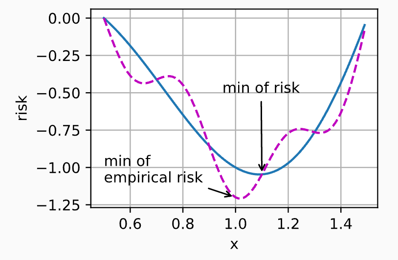
The figure above, from D2L, illustrates the relationship between \(f\) and \(g\). It reflects a reality: \(g\) is always less smooth than \(f\).

• \(f\) is perfectly smooth: Because \(f\) encompasses infinitely many real data points. In statistics, as the amount of data approaches infinity, the influence of individual extreme data points (noise) is thoroughly diluted and smoothed out. Therefore, the surface of \(f\) as a function of parameters \(w\) is very smooth, and its minimum represents the absolute truth.
• \(g\) is bumpy and uneven: Your training set has only a finite number of \(n\) samples. If this batch happens to contain a few rare edge cases or data with significant noise, the computation of \(g\) will be heavily skewed by these outliers. On the function surface, \(g\) will be riddled with local depressions (local optima), spikes, and steep slopes.

Having understood the difference between \(f\) and \(g\), the "division of labor and tension" between deep learning and optimization algorithms becomes very clear:

The sole objective of optimization is to minimize the empirical risk \(g\).

Optimization algorithms (such as SGD or Adam) lack any "big picture" awareness. They cannot see the real world outside — they can only see the tens of thousands of training images you feed them. Their task is purely to play a mathematical game: adjust parameters to drive the training set error as low as possible.

However, deep learning is concerned with generalization. We train models not to perfectly memorize problems already seen (the training set), but to give accurate answers when facing entirely new, unseen problems (the test set or real deployment scenarios). Therefore:

The ultimate goal of deep learning is to minimize the risk \(f\).

In an ideal scenario, if training data were infinite, \(g\) would equal \(f\). But in reality, data is always finite, so the empirical risk \(g\) is only a rough, noisy approximation of the risk \(f\) (i.e., "less smooth than \(f\)" as mentioned above). When we push the optimizer too hard and squeeze \(g\) to its extreme, the model begins to memorize the idiosyncrasies and noise in the training set. At this point, although \(g\) has been driven very low, the real-world risk \(f\) actually surges. This explains why reducing training error does not necessarily equate to reducing generalization error.

To prevent the optimizer from driving \(g\) so low that it harms \(f\), deep learning introduces many specialized techniques — such as regularization (weight decay), early stopping, and dropout. These techniques may seem "counterintuitive" from a pure mathematical optimization standpoint because they actually hinder the optimizer from driving \(g\) to its absolute minimum. Yet they effectively protect the model, bringing it closer to the true \(f\).

From this perspective:

Deep Learning = Optimization + Regularization

Of course, deep learning is also influenced by data and architecture, so the complete picture is: Deep Learning = Data + Architecture + Optimization + Regularization.

However, viewed solely from the perspective of risk function \(f\) and empirical risk function \(g\), optimization and regularization together aim to achieve Structural Risk Minimization (SRM):

\[ J(w) = g(w) + \lambda R(w) \]

where

\[ g(w) = \frac{1}{n} \sum_{i=1}^n \ell(w; x_i, y_i) \]

is the empirical risk function (the average error on the training set) mentioned above, measuring how well the model fits the current training data. The job of optimization algorithms (Adam, SGD, etc.) is to drive this term toward 0. We can think of this as the engine's output (empirical risk).

\(R(w)\) is the braking force (regularization / penalty term) — a mathematical function that measures model complexity. The most common example is \(L_2\) regularization (weight decay), whose formula is \(R(w) = \|w\|^2\). It measures the model's complexity or "ambition." The larger the parameter values \(w\), the harder the model is contorting itself to accommodate the data (including noise). The purpose of \(R(w)\) is to penalize overly complex models with excessively large weights. It tells the optimizer: "You may fit the data, but you must not make drastic moves — stay smooth and simple."

\(\lambda\) (Lambda) is a positive constant set by the practitioner. It determines whether the engine or the brake has the final say. If \(\lambda = 0\), the brake is completely disengaged, degenerating into pure empirical risk minimization (rote memorization, guaranteed overfitting). If \(\lambda\) is very large, the brake is fully engaged: the model dares not move at all (weights are all pushed to 0, nothing is learned, underfitting).

Putting all of this together, we touch upon the soul of machine learning theory — the generalization bound. In statistical learning theory, mathematicians have proved a remarkable inequality. For the true risk \(f(w)\) and empirical risk \(g(w)\), the following relationship holds:

\[ f(w) \le g(w) + \text{complexity penalty term} \]

This inequality tells us: The real-world error \(f(w)\) is jointly bounded by "training set error" and "model complexity."

• If the model is too complex, even though \(g(w)\) drops to 0, the "complexity penalty term" explodes, causing the true generalization error \(f(w)\) to remain high (this is the mathematical essence of overfitting).
• To bring the true \(f(w)\) down, we cannot look at \(g(w)\) alone — we must minimize both terms on the right-hand side simultaneously!

Therefore, what deep learning truly optimizes — \(J(w) = g(w) + \lambda R(w)\) — is in fact directly optimizing an upper bound on the true risk \(f(w)\). By forcibly injecting \(R(w)\) into the optimization objective, we mathematically "trick" the optimizer (which only knows how to find the lowest point) into finding a perfect balance between "fitting the data" and "staying simple," thereby safely arriving at the valley of the true risk \(f(w)\)**.

In PyTorch, this profound mathematical concept is encapsulated with remarkable elegance:

optimizer = torch.optim.SGD(model.parameters(), lr=0.01, weight_decay=1e-4)

Or using the Adam optimizer:

optimizer = torch.optim.Adam(model.parameters(), lr=0.001, weight_decay=1e-4)

In this line of code, the mathematical formula \(J(w) = g(w) + \lambda R(w)\) is decomposed into several concrete control knobs:

• model.parameters() (target): Tells the optimizer engine which weight parameters \(w\) to adjust.
• lr=0.01 (throttle): The learning rate, determining how large a step the engine takes in the direction of reducing \(g(w)\) each time.
• weight_decay=1e-4 (brake): This is our mathematical parameter \(\lambda\)! In PyTorch, \(L_2\) regularization is called Weight Decay. The value 1e-4 (0.0001) set here is the braking intensity.

It is worth noting that PyTorch calls L2 regularization "weight_decay" because a very clever engineering implementation detail is hidden here. In pure mathematical theory, we add the regularization term to the loss function:

\[ J(w) = \text{Loss} + \frac{\lambda}{2} \|w\|^2 \]

When you differentiate this total objective \(J(w)\) (compute the gradient), the original loss function yields \(\nabla g\), while the regularization term differentiates with respect to \(w\) to give exactly \(\lambda w\).

So, the actual mathematical computation at each parameter update is:

\[ w_{\text{new}} = w_{\text{old}} - \text{lr} \times (\nabla g + \lambda w_{\text{old}}) \]

Rearranging slightly:

\[ w_{\text{new}} = (1 - \text{lr} \times \lambda) w_{\text{old}} - \text{lr} \times \nabla g \]

See what is happening? Under the hood, PyTorch never bothers computing the sum of squares (\(\|w\|^2\)). It simply multiplies the current weights \(w\) by a number slightly less than 1 (e.g., \(0.9999\)) before each update, causing the weights to "decay" slightly, and then subtracts the normal gradient.

It is as if the optimizer is pulling the weights upward (fitting the data), while weight_decay acts like a spring constantly pulling the weights back toward \(0\) (keeping things simple). This approach of directly intervening at the gradient update step is both efficient and a perfect realization of the mathematical effect of \(L_2\) regularization.

For detailed coverage of weight decay, dropout, and other techniques, see the Regularization notes.

.

Bias and Variance

In machine learning (and deep learning), we are always pursuing the smallest "total error." We can decompose the total error into bias and variance:

• Bias \(\approx\) error on the training set. Bias measures the gap between the expected prediction of the model and the true value. High bias means the model performs poorly even on the training set (large error). This typically indicates underfitting — the model is too simple and fails to capture the patterns in the data.
• Variance \(\approx\) the difference between test set error and training set error. Variance measures the spread (stability) of the model's predictions. High variance means the model performs well on the training set but poorly on the test set (large error). This typically indicates overfitting — the model has memorized training set noise rather than general patterns.

Mathematically, suppose the true function we want to predict is \(y = f(x) + \epsilon\), where \(\epsilon\) is random noise (mean 0, variance \(\sigma^2\)). Our trained model is \(\hat{f}(x)\). For a specific point \(x\), the expected prediction error can be decomposed as:

\[ E[(y - \hat{f}(x))^2] = \text{Bias}[\hat{f}(x)]^2 + \text{Var}[\hat{f}(x)] + \sigma^2 \]

Computing Bias:

\[ \text{Bias}[\hat{f}(x)] = E[\hat{f}(x)] - f(x) \]

Bias measures the gap between the expected prediction of the model and the true value. If you train 100 models using different training data, it indicates how far the average prediction of these 100 models deviates from the truth.

Computing Variance:

\[ \text{Var}[\hat{f}(x)] = E[(\hat{f}(x) - E[\hat{f}(x)])^2] \]

Variance measures the spread (stability) of the model's predictions — how much the predictions fluctuate when the training set changes slightly.

Optimization and Regularization

In deep learning, optimization is the process of finding a set of model parameters that minimizes the loss function. Simply put, every machine learning model is essentially searching for a parameter set that minimizes the loss function; the optimization process is the continual adjustment of parameters to minimize that loss.

In other words, most models can be decomposed into:

• Model architecture: determines how you go from input data to predictions
• Loss function: defines the evaluation criterion for results
• Optimization algorithm: determines how to find the parameter set that minimizes the loss

A complete deep learning model (neural network) training process can be understood as follows:

* Split the dataset into portions and train over multiple epochs; input normalization (**Input Normalization**) is applied here
* Before starting the loop, initialize the neural network parameters $\theta$ (**Initialization**)
* Before each epoch, adjust the learning rate (**Learning Rate Scheduling**), then enter the epoch (note: in practice, this is usually done after the epoch):
  1. Within each epoch, load data in batches (**Batching**):
     1. Forward propagation: feed data into the model to obtain predictions
        * **Batch Normalization** can be applied here
        * **Regularization** can be applied here, e.g., Dropout — randomly deactivating neurons during propagation to prevent rote memorization
     2. Compute the loss from the forward pass predictions and true values
        * **Regularization** can be applied here, e.g., L2 weight decay
     3. Update parameters using optimization:
        1. Zero out residual gradients from the previous batch
        2. Backpropagation: compute the gradient of the current loss with respect to each parameter via the chain rule
        3. The **Optimizer** modifies parameters $\theta$ based on gradients and learning rate (i.e., optimization)
* After the epoch, evaluate on the validation set; if performance is good, save the parameters so that if overfitting occurs or training is interrupted later, we can roll back to the best-performing version

The items I highlighted above — Initialization, Learning Rate Scheduling, Batching, Normalization, Optimizer — are all aimed at helping the loss function find its minimum faster, more stably, and more effectively, and thus all fall under the umbrella of Optimization.

Although most optimization techniques aim to find the minimum of the loss function, Regularization is special in that it deliberately interferes with optimization. This interference trades some training performance for lower loss on unseen test data, thereby preventing overfitting.

While regularization is not optimization per se, optimization and regularization together form the core of model training, so we study them together.

If we liken optimization to descending a mountain to find the lowest valley, then each of the above techniques serves the following role:

1. Initialization: The starting point of optimization (determines where on the mountain you begin your descent)
2. Batching: The sampling strategy for optimization (determines how much terrain you observe before deciding your next step)
3. Regularization: Constraints on optimization (prevents you from taking shortcuts that lead into dead ends of the training data)
4. Optimizer: The execution of optimization (how your feet move in response to terrain feedback)
5. Learning Rate Scheduling: Pace control for optimization (determines how stride length should change as you approach the destination)
6. Normalization: Terrain smoothing for optimization (smooths rugged mountain paths to be even and gradual, preventing slipping on steep slopes or getting stuck on flat ground)

Mathematical Representation of DNNs

A deep neural network (DNN) can be precisely described using a layer-wise recursive mathematical formulation (cf. Tufts CS130 Topic2). For an \(L\)-layer DNN, the computation at layer \(\ell\) is:

\[ h^{(\ell)} = g^{(\ell)}\!\left(W^{(\ell)T} h^{(\ell-1)} + b^{(\ell)}\right), \quad \ell = 1, 2, \ldots, L \]

where:

• \(h^{(\ell)} \in \mathbb{R}^{n_\ell}\): the output (hidden representation) of layer \(\ell\), with \(h^{(0)} = x\) as the input
• \(W^{(\ell)} \in \mathbb{R}^{n_{\ell-1} \times n_\ell}\): the weight matrix of layer \(\ell\)
• \(b^{(\ell)} \in \mathbb{R}^{n_\ell}\): the bias vector of layer \(\ell\)
• \(g^{(\ell)}(\cdot)\): the activation function of layer \(\ell\) (e.g., ReLU, Sigmoid, Tanh)

The entire network can be expressed as a function composition:

\[ f(x; \theta) = g^{(L)} \circ g^{(L-1)} \circ \cdots \circ g^{(1)}(x) \]

where \(\theta = \{W^{(1)}, b^{(1)}, \ldots, W^{(L)}, b^{(L)}\}\) is the collection of all trainable parameters.

DNN training as an optimization problem: Given a dataset \(\mathcal{D} = \{(x_i, y_i)\}_{i=1}^{N}\), training a DNN amounts to solving:

\[ \min_\theta \frac{1}{N} \sum_{i=1}^{N} L\!\left(f(x_i; \theta),\; y_i\right) \]

where \(L(\cdot, \cdot)\) is the loss function. This optimization problem has the following characteristics:

• High-dimensional: The parameter \(\theta\) can have dimensions in the millions or even billions
• Non-convex: Due to the nonlinearity of activation functions and the composition of layers, the objective function is almost always non-convex
• Stochastic: In practice, mini-batches are used to approximate the full gradient, introducing stochasticity

Surrogate Loss Functions

In classification tasks, what we truly care about is the 0-1 loss (misclassification rate):

\[ L_{0\text{-}1}(f(x;\theta), y) = \mathbb{1}[f(x;\theta) \neq y] \]

However, the 0-1 loss is non-differentiable (a step function) and cannot be directly optimized with gradient descent. Therefore we use a surrogate loss function — a differentiable substitute whose minimization indirectly minimizes the true 0-1 loss.

Cross-entropy loss is the most commonly used surrogate loss for classification. It derives from minimizing the KL divergence:

\[ D_{KL}(p \| q) = \sum_{k} p(k) \log \frac{p(k)}{q(k)} = -H(p) - \sum_{k} p(k) \log q(k) \]

where \(p\) is the true distribution (one-hot labels) and \(q\) is the model's predicted distribution (softmax output). Since \(H(p)\) is a constant (equal to 0) for one-hot labels, minimizing the KL divergence is equivalent to minimizing the cross-entropy:

\[ L_{CE} = -\sum_{k=1}^{C} y_k \log \hat{y}_k \]

For binary classification, this simplifies to: \(L_{BCE} = -[y \log \hat{y} + (1-y) \log(1-\hat{y})]\)

Loss functions for regression tasks:

• Mean Squared Error (MSE): \(L_{MSE} = \frac{1}{N}\sum_{i=1}^{N}(f(x_i;\theta) - y_i)^2\), penalizes large errors more heavily, sensitive to outliers
• Mean Absolute Error (MAE): \(L_{MAE} = \frac{1}{N}\sum_{i=1}^{N}|f(x_i;\theta) - y_i|\), more robust to outliers, but non-differentiable at zero

Gradient Descent Fundamentals

Chapter 4 of Ian Goodfellow's classic textbook covers not only numerical computation, gradient descent, and the Hessian, but also several other concepts such as optimal step size, Newton's method, Lipschitz continuity, and convex optimization. These will be revisited if encountered later. There are too many concepts to memorize all at once, so for now, let us remember the most important ones:

• The gradient is a vector that always points in the direction of steepest function increase
• Gradient descent simply moves in the opposite direction of the gradient
• The Hessian matrix describes the curvature (degree of bending) of the terrain. By analyzing the Hessian, we can determine whether the current position is a U-shaped valley (low curvature), a V-shaped canyon (high curvature), or a more complex saddle point
• When the maximum and minimum curvatures of the Hessian matrix differ drastically, we encounter ill-conditioned terrain. This terrain resembles a canyon with steep walls and a flat floor, causing gradient descent to converge slowly, oscillating back and forth across the canyon — the number-one enemy of all optimization algorithms
• The first-order Taylor expansion proves why the negative gradient direction is effective; the second-order expansion reveals how curvature affects optimization performance and exposes the gap between linear prediction and reality
• In the high-dimensional spaces of deep learning, the vast majority of zero-gradient points are saddle points, not local minima. Simple gradient descent gets stuck at these points, while modern optimizers (to be studied later) have mechanisms to escape saddle points
• Since the Hessian describes the terrain, the ideal optimization approach would simultaneously use both the gradient and the Hessian at each step to compute the perfect next move. Newton's method achieves this perfectly but is prohibitively expensive for deep learning — yet it remains the target that all advanced optimizers try to imitate and approximate

There is one more section at the end of Chapter 4 in Ian's book — "Constrained Optimization" — which we will skip for now. Our current focus is on unconstrained optimization, whose goal is to find the minimum of a function in an unrestricted, open space; this is the standard scenario for training most deep neural networks such as CNNs, RNNs, and Transformers.

An important related branch — constrained optimization (the section in the book) — aims to find the minimum of a function subject to a set of rules or constraints. The technical approach here involves KKT conditions and related methods, which are more important in specific machine learning methods such as SVMs and certain specialized deep learning topics.

Since our current focus is on unconstrained optimization, we will skip this section for now and return to it when needed.

Next, I will introduce various gradient descent optimizers. First, based on whether they use first-order or second-order information, optimizers can be broadly divided into two categories: first-order optimizers and second-order optimizers.

First-Order Optimizers, listed in chronological order of development:

1. Plain gradient descent: Gradient Descent (1847), SGD (1951)
2. With momentum: Polyak Momentum (1964), Nesterov Momentum (1983)
3. With adaptive learning rate: AdaGrad (2011), RMSProp (2012), AdaDelta (2012)
4. Combining both momentum and adaptive gradients: Adam (2014), AdamW (2017)

Second-Order Optimizers, listed in chronological order of development:

1. Pure second-order: Newton's method (17th century), Quasi-Newton L-BFGS (1989)
2. Approximate second-order: KFAC (2015), AdaHessian (2020)

For detailed coverage of specific optimizers, see the Optimizer notes.

Gradient

The gradient is the most fundamental mathematical concept in machine learning and the cornerstone of optimization algorithms. In machine learning, our goal is typically to find a mathematical model that minimizes the "error" when processing data. This search for a minimum is the optimization problem. Imagine you are at the top of a mountain and want to reach the base as quickly as possible. If you know which direction is "downhill" at every position, you can keep stepping forward until all surrounding directions are "uphill" — at which point you have found a local minimum. The gradient is the tool that tells you the direction and magnitude of the fastest function change at the current position.

For a scalar function \(f(\boldsymbol{x})\) with a multi-dimensional vector input \(\boldsymbol{x} = (x_1, x_2, \dots, x_n)^\top\), its gradient at \(\boldsymbol{x}\) is defined as:

\[ \nabla_{\boldsymbol{x}} f(\boldsymbol{x}) = \left( \frac{\partial f}{\partial x_1}, \frac{\partial f}{\partial x_2}, \dots, \frac{\partial f}{\partial x_n} \right)^\top \]

Each component of the gradient is the partial derivative of the function with respect to that dimension's variable. The gradient itself is a vector whose dimensionality matches that of the independent variable \(\boldsymbol{x}\).

The gradient vector \(\nabla f\) points in the direction of steepest increase of the function at that point. Geometrically, the gradient vector is always perpendicular to the function's level curves (or level surfaces). Since the gradient points in the direction of steepest increase, its opposite direction (negative gradient) is the direction of steepest decrease. This is precisely why gradient descent updates parameters along the negative gradient direction.

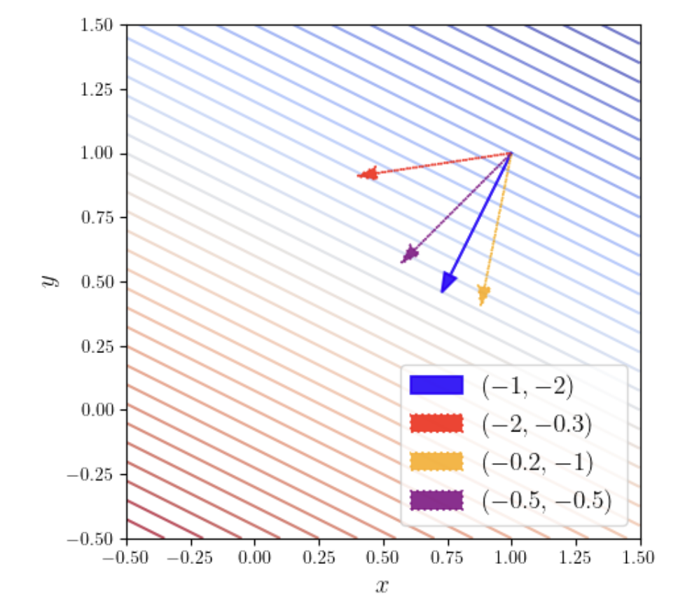
The figure above shows the gradient of the function \(f(x, y) = -x - 2y\) at the point \((1, 1)\). The parallel diagonal lines in the figure are level curves, each representing a set of points where the function has equal value. As can be seen, the blue arrow crosses the most level curves, meaning that for the same step length (arrow length), the blue arrow (gradient direction) crosses the most contour lines — indicating that this is the direction along which the function increases most rapidly.

The conclusion that "the gradient points in the direction of steepest increase" holds for nonlinear functions as well. For nonlinear functions, using the intuition from the single-variable Taylor expansion, a multivariate function near a point \(\boldsymbol{x}_0\) can also be linearly approximated:

\[ f(\boldsymbol{x}) \approx f(\boldsymbol{x}_0) + \nabla f(\boldsymbol{x}_0)^\top (\boldsymbol{x} - \boldsymbol{x}_0) \]

This means that as long as we look at a sufficiently small (local) region, any smooth complex function looks like a "flat plane" (linear function). Therefore, at that point, the gradient still points in the direction of steepest increase.

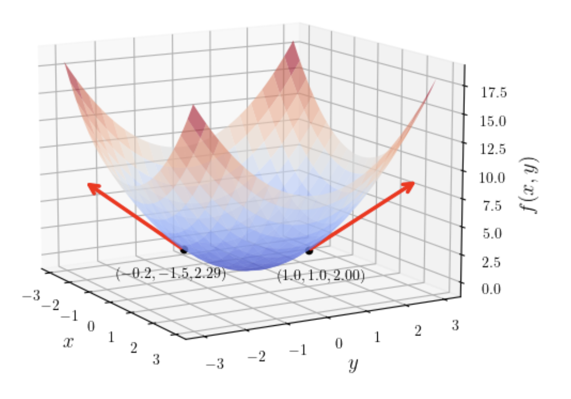
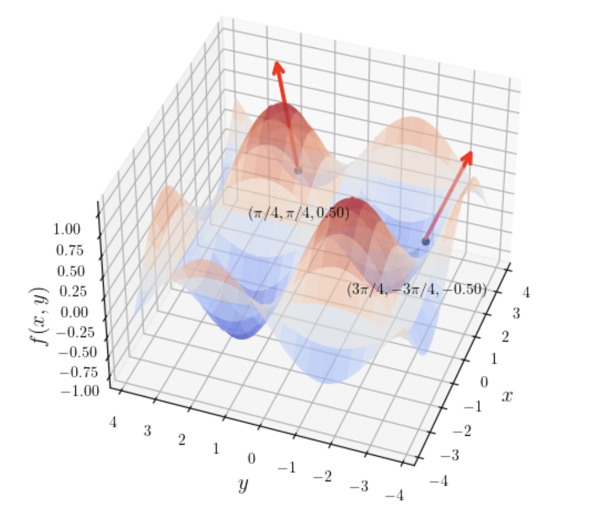
Paraboloid (\(f(x, y) = x^2 + y^2\)): Shaped like a bowl; the gradient points radially away from the center.

Saddle surface (\(f(x, y) = x^2 - y^2\)): Shaped like a saddle; the gradient direction changes dramatically across different regions.

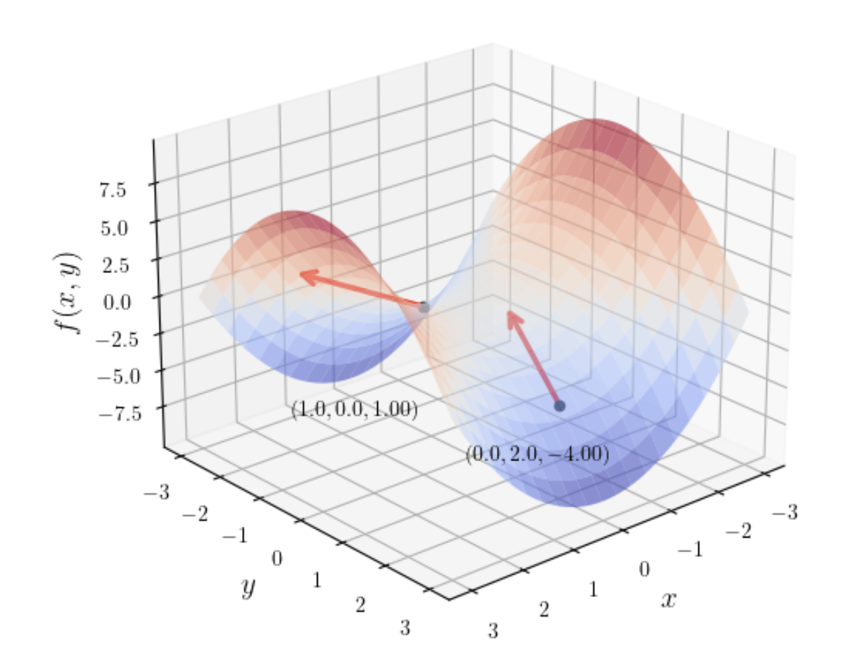
Sine product surface (\(f(x, y) = \sin(x)\sin(y)\)): Resembles an undulating egg carton; the gradient points toward various "peaks."

When working with loss functions, the following formulas are frequently used:

• Derivative of a linear function:
  • \(\nabla_{\boldsymbol{x}} (\boldsymbol{y}^\top \boldsymbol{x}) = \boldsymbol{y}\)
  • \(\nabla_{\boldsymbol{x}} (\boldsymbol{x}^\top \boldsymbol{y}) = \boldsymbol{y}\)
  • \(\nabla_{\boldsymbol{x}} (\boldsymbol{A}\boldsymbol{x}) = \boldsymbol{A}^\top\)
• Derivative of a quadratic form:
  • \(\nabla_{\boldsymbol{x}} (\boldsymbol{x}^\top \boldsymbol{x}) = 2\boldsymbol{x}\)
  • \(\nabla_{\boldsymbol{x}} (\boldsymbol{x}^\top \boldsymbol{A} \boldsymbol{x}) = (\boldsymbol{A} + \boldsymbol{A}^\top)\boldsymbol{x}\)
• Norms and constants:
  • \(\nabla_{\boldsymbol{x}} \|\boldsymbol{x}\|_2 = \frac{\boldsymbol{x}}{\|\boldsymbol{x}\|_2}\)
  • \(\nabla_{\boldsymbol{x}} (a\boldsymbol{x}) = a\boldsymbol{I}\) (where \(a\) is a scalar and \(\boldsymbol{I}\) is the identity matrix)

For saddle points, even if the gradient \(\nabla f(\boldsymbol{x}) = \mathbf{0}\), the point is not necessarily an extremum (as with the saddle surface). The Hessian matrix \(\boldsymbol{H}_f\) must be examined to make a definitive determination. Details are covered in later sections.

Gradient Descent

In mathematics, optimization refers to the process of systematically selecting and finding the best solution(s) from all possible alternatives. Applied to functions, it generally means changing \(x\) to minimize \(f(x)\); maximization is essentially minimization, since we can minimize \(-f(x)\) using the same methods.

We call the function to be minimized the objective function or criterion. When we are minimizing it, this function is also sometimes called the cost function, loss function, or error function. Different contexts or papers may favor one name over another, but they all refer to the same thing — the target function to be minimized.

For the value of \(x\) that achieves the function's minimum, we write \(x^{*} = \arg\min f(x)\). For maximization, \(x^{*} = \arg\max_{x} f(x)\). In calculus, for the function \(y=f(x)\), its derivative is denoted \(f'(x)\) or \(\frac{dx}{dy}\). If \(f'(x)>0\), it means the function is sloping upward at \(x\) — the trend is increasing, meaning the function is still growing at that point. Conversely, if the derivative is negative, the trend is decreasing.

Since our goal is to find the function's minimum:

• When the derivative is positive, the function is "uphill" — we should decrease \(x\), moving against the uphill direction
• When the derivative is negative, the function is "downhill" — we should increase \(x\), continuing downhill

This strategy is called gradient descent. Gradient descent is the earliest gradient-based algorithm, proposed by mathematician Augustin-Louis Cauchy in 1847. Stochastic gradient descent is a practical improvement upon gradient descent: instead of computing the average gradient over all samples, it randomly selects one (or a small batch of) sample(s) to estimate the gradient and update parameters. This makes it converge much faster than the traditional method on modern large-scale datasets (such as in deep learning), and it can escape some local traps.

Mathematically, the first-order Taylor expansion proves why gradient descent is effective:

\[ f(x+\epsilon) \approx f(x) + \epsilon f'(x) \]

This expression states that at \(x\), if we move a tiny distance \(\epsilon\), the function value after moving is approximately the original function value at \(x\) plus the derivative at \(x\) times this tiny distance. To make the new function value \(f(x+\epsilon)\) less than the old value \(f(x)\), we simply need the incremental term \(\epsilon f'(x)\) to be negative. The most effective way to ensure this term is negative is to choose our "travel direction" \(\epsilon\) with the opposite sign of the derivative \(f'(x)\). In other words, the first-order Taylor expansion proves that gradient descent is an effective strategy.

When \(f'(x)=0\), the derivative provides no information about which direction to move, so such a point is called a critical point or stationary point.

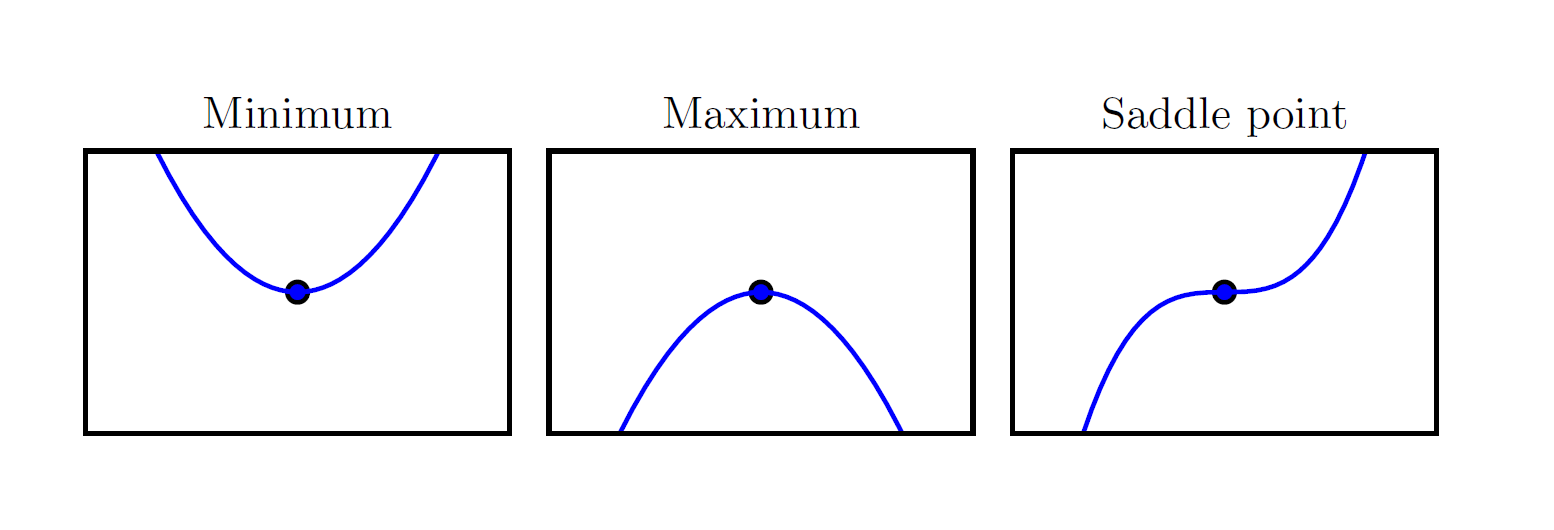
As shown in the figure above, when the derivative is zero, three scenarios are possible:

• Local Minimum
• Local Maximum
• Saddle Point (also called an Inflection Point)

In these three scenarios, we use the second derivative to determine which case we are in:

• If the second derivative \(f''(x)>0\), the function is concave up — a valley, a local minimum
• If the second derivative \(f''(x)<0\), the function is concave down — a peak, a local maximum
• If the second derivative \(f''(x)=0\), the function is flat — like the center of a saddle

In gradient descent, a local minimum is the ideal stopping point, indicating that we have found a potential solution. Both local maxima and saddle points are undesirable stopping points, because at these points we cannot determine the correct direction to proceed. Standard gradient descent cannot distinguish among these three cases — it stops whenever the gradient is zero. Modern optimization algorithms have therefore developed strategies such as momentum, stochasticity, and second-order methods to address the problems of maxima and saddle points.

Our ultimate goal is to find the global minimum. A function may have one global minimum, multiple global minima, or no global minimum at all. Consider a function that goes to positive infinity on the left and negative infinity on the right, such as \(f(x) = -x^3 + 3x\):

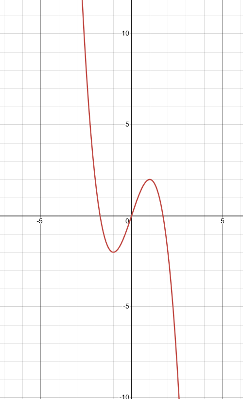
The function above tends toward negative infinity on the right side — mathematically called unbounded below. In gradient descent, such functions lead to divergence: the optimization process fails to converge to a stable solution and instead tends toward an invalid or infinite result. Divergence can also occur when function values tend toward positive infinity — for example, if the learning rate (discussed shortly) is set too high, the step is too large, overshooting the valley minimum to a higher position on the other side. The next step, trying to descend, overshoots even further, causing the trajectory to climb ever higher.

Now let us formally examine how gradient descent is applied in deep learning. Everything discussed above concerned one-dimensional functions — a single curve — but in practice we always deal with multivariable functions.

For a function \(f: \mathbb{R}^n \to \mathbb{R}\) with multi-dimensional input (where \(\mathbb{R}^n\) means the input is an \(n\)-dimensional vector), the notion of a minimum has a clear requirement: the minimum must be a scalar. This is because scalars can be directly compared, whereas vectors cannot. This scalar is commonly referred to as the loss or cost.

At the minimum, there is a corresponding \(n\)-dimensional vector — this specific vector is our optimal solution. In other words, the criterion for whether a vector is an optimal solution is to substitute it into the function and check whether the resulting scalar is the smallest among all possible outcomes.

For one-dimensional functions, we already know that differentiating the function and finding where the derivative equals zero yields a special point that could be a minimum, maximum, or saddle point. For multi-dimensional vectors, we differentiate the function using partial derivatives to obtain a "vector of all partial derivatives" — the gradient — denoted \(\nabla_{x} f(x)\), read as "the gradient with respect to \(x\)." The \(i\)-th element of the gradient is the partial derivative of \(f\) with respect to \(x_i\). In the multi-dimensional case, a critical point is one where all elements of the gradient are zero.

---

As an example, suppose our multivariable function is \(f(x, y) = x^{2} + 2xy + y^{3}\). The input vector is:

\[ \mathbf{x} = \begin{bmatrix} x \\ y \end{bmatrix} \]

Our goal is to compute the gradient of this function at any point \((x,y)\). By definition, for our two-dimensional function, the gradient is the vector containing all partial derivatives:

\[ \nabla_{X} f(x, y) = \begin{bmatrix} \text{partial derivative w.r.t. }x \\ \text{partial derivative w.r.t. }y \end{bmatrix} = \begin{bmatrix} \dfrac{\partial f}{\partial x} \\ \dfrac{\partial f}{\partial y} \end{bmatrix} \]

Through computation, we obtain the partial derivative with respect to \(x\):

\[ \frac{\partial f}{\partial x} = 2x + 2y \]

and the partial derivative with respect to \(y\):

\[ \frac{\partial f}{\partial y} = 2x + 3y^{2} \]

Substituting both partial derivatives back into the vector structure from the first step:

\[ \nabla_{X} f(x, y) = \begin{bmatrix} 2x + 2y \\ 2x + 3y^{2} \end{bmatrix} \]

This is the gradient formula for function \(f(x,y)\) at any point \((x,y)\). Using this formula, you can quickly compute the gradient vector at any point by substituting its coordinates.

For example, at point \((3,2)\):

\[ \nabla_{X} f(x=3, y=2) = \begin{bmatrix} 10 \\ 18 \end{bmatrix} \]

This gradient vector means that the direction of steepest increase of \(f\) is along 10 units in the \(x\)-axis and 18 units in the \(y\)-axis simultaneously. In two dimensions, we can visualize this by drawing a plot, but for a 10,000-dimensional vector, we simply apply the same principle without needing to plot anything. In other words, using this method, for vectors of arbitrary dimension, we can determine the gradient landscape at a point without drawing any figures.

For the direction described above, we know it points in the direction of steepest increase of \(f\) — the steepest uphill path. In gradient descent, to make the function decrease as fast as possible, we move in the opposite direction of this gradient — i.e., move a small step in the \(\begin{bmatrix}-10 \\-18\end{bmatrix}\) direction.

---

The derivative of a single-variable function and the gradient vector of a multivariable function share the same property: each component is an "uphill guide," indicating the direction and intensity of function increase along its respective dimension. This is a property of derivatives. Therefore, for the gradient vector, combining all dimensions' "uphill guides" into a resultant direction necessarily yields the direction of steepest overall increase. The textbook confirms this through a mathematical proof based on directional derivatives to find the direction of fastest function decrease (pp. 76-77), which we will not expand upon here. We only need to remember: The gradient always points in the direction of steepest ascent; its opposite direction is the steepest descent.

Now that we know the downhill direction, we can proceed along it to search for the minimum. First, we specify a fixed positive scalar step size, denoted \(\epsilon\), called the learning rate.

For a multi-dimensional vector \(X\):

\[ X_{t+1} = X_t - \epsilon \nabla_{X} f(X_t) \]

This formula is the update rule for the method of steepest descent, or equivalently, gradient descent.

Through this iterative steepest descent formula, we can keep finding the downhill path until we reach a completely flat location. We can iteratively approach the target, or directly solve the system of equations equal to 0 to jump straight to the critical point (this direct approach is called the analytical solution). In the real world, the loss functions of deep learning models are often extremely complex and the gradient equation systems are enormous, making analytical solutions impossible. This is why we need gradient descent — an approach that may seem clumsy but is remarkably effective as an iterative method.

Gradient descent can only be used for optimization problems in continuous spaces. However, for many problems with discrete parameters — such as integer programming and the traveling salesman problem — although we cannot directly compute gradients, we can use a similar idea: continually finding the best direction at the current position and moving a small step to find the optimum. This method is called the hill climbing algorithm. (It is called "hill climbing" because the algorithm is often used for maximizing objective functions, such as in board games and genetic algorithms; gradient descent is mainly used in machine learning tasks, where our goal is almost always to minimize the loss function.)

---

Jacobian

In the discussion of gradient descent above, we mentioned using a scalar to measure the minimum (i.e., the loss value \(L\)) of an input function (such as a multi-dimensional vector containing all neural network parameters \(x\)), written as \(f: \mathbb{R}^n \to \mathbb{R}\).

However, even though our neural network ultimately produces a scalar, the intermediate layers of the network involve multiple multi-dimensional-input-to-multi-dimensional-output transformations, as shown below:

This intermediate process is written as \(f: \mathbb{R}^n \to \mathbb{R}^m\), meaning \(n\)-dimensional input to \(m\)-dimensional output. For such intermediate layers, how do we understand how each input's change affects each output? Using gradient vectors, for each output variable we would need to compute \(n\) partial derivatives; for \(m\) output variables, that amounts to \(m \times n\) partial derivatives. How do we organize these \(m \times n\) partial derivatives to systematically represent and use this massive amount of derivative information? The Jacobian matrix was created precisely to solve this problem.

The Jacobian matrix provides a perfect, compact mathematical structure — a single matrix that neatly stores all \(m \times n\) partial derivatives. With this organization, we can then leverage matrix multiplication from linear algebra to express and compute the chain rule concisely and efficiently.

Specifically, suppose we have a function \(f\) that takes an \(n\)-dimensional vector input

\[ x = [x_1, x_2, \ldots, x_n]^T \]

and produces an \(m\)-dimensional vector output

\[ y = f(x) = [f_1(x), f_2(x), \ldots, f_m(x)]^T. \]

Here \(f_1, f_2, \ldots, f_m\) are \(m\) independent functions that together compose the multi-dimensional output.

The Jacobian matrix (usually denoted \(\mathbf{J}\)) arranges all first-order partial derivatives of all output functions with respect to all input variables into a matrix. Its standard form is:

\[ \mathbf{J} = \begin{bmatrix} \dfrac{\partial f_1}{\partial x_1} & \dfrac{\partial f_1}{\partial x_2} & \cdots & \dfrac{\partial f_1}{\partial x_n} \\ \dfrac{\partial f_2}{\partial x_1} & \dfrac{\partial f_2}{\partial x_2} & \cdots & \dfrac{\partial f_2}{\partial x_n} \\ \vdots & \vdots & \ddots & \vdots \\ \dfrac{\partial f_m}{\partial x_1} & \dfrac{\partial f_m}{\partial x_2} & \cdots & \dfrac{\partial f_m}{\partial x_n} \end{bmatrix}. \]

In this matrix:

• Each row represents the partial derivatives of one output function with respect to all input variables; you can view the \(i\)-th row as the (transposed) gradient of function \(f_i\).
• Each column represents the partial derivatives of all output functions with respect to one input variable.

---

Here is a concrete example of a mapping from \(\mathbb{R}^2\) to \(\mathbb{R}^3\). Suppose the input vector is

\[ x = \begin{bmatrix} x_1 \\ x_2 \end{bmatrix}. \]

The output vector is defined by the following three functions:

\[ f_1(x_1, x_2) = x_1^2 + 5x_2 \]

\[ f_2(x_1, x_2) = 3x_1 \sin(x_2) \]

\[ f_3(x_1, x_2) = x_1^2 x_2 \]

By definition, the Jacobian matrix \(\mathbf{J}\) for this function will be a \(3 \times 2\) matrix. Let us compute its elements row by row:

First row (partial derivatives of \(f_1\)):

• \[ \dfrac{\partial f_1}{\partial x_1} = 2x_1 \]
• \[ \dfrac{\partial f_1}{\partial x_2} = 5 \]

Second row (partial derivatives of \(f_2\)):

• \[ \dfrac{\partial f_2}{\partial x_1} = 3\sin(x_2) \]
• \[ \dfrac{\partial f_2}{\partial x_2} = 3x_1\cos(x_2) \]

Third row (partial derivatives of \(f_3\)):

• \[ \dfrac{\partial f_3}{\partial x_1} = x_2^2 \]
• \[ \dfrac{\partial f_3}{\partial x_2} = 2x_1x_2 \]

Filling these results into the matrix, we obtain the Jacobian matrix expression for this function:

\[ \mathbf{J} = \begin{bmatrix} 2x_1 & 5 \\ 3\sin(x_2) & 3x_1\cos(x_2) \\ x_2^2 & 2x_1x_2 \end{bmatrix}. \]

This matrix completely describes how small changes in the input vector propagate to and affect the output vector at any point \((x_1, x_2)\).

---

Hessian

In gradient descent, we find the steepest direction and then descend in the opposite direction. We set a learning rate to determine the step size. This leads to a natural question: when we descend, does the actual decrease in height match our expectation?

To check whether a gradient descent step achieves the expected outcome, we need to examine the curvature of the descent.

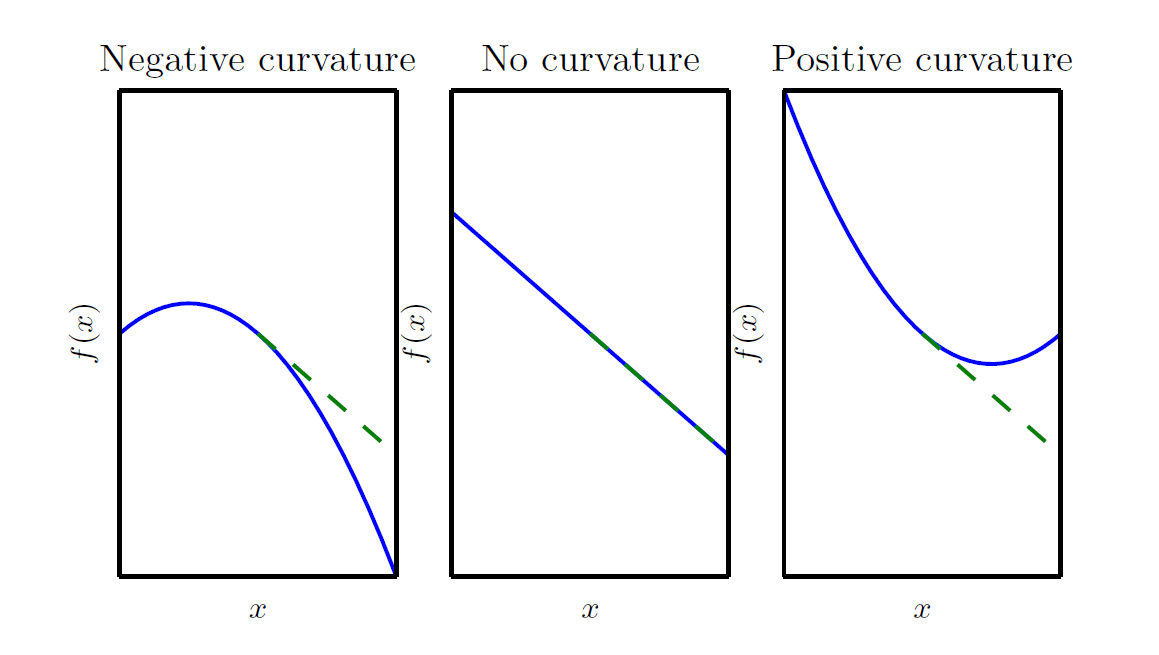
In the three scenarios shown above, the green dashed line represents the first-order Taylor expansion \(f(x+\epsilon) \approx f(x) + \epsilon f'(x)\) mentioned earlier — the linear prediction that the gradient descent algorithm relies on. Based on this prediction, we obtain the new position \(x_{\text{new}} = x - \eta f'(x)\).

Notice that the first-order Taylor expansion uses an approximation sign, meaning it is only an estimate that ignores higher-order information. What is ignored is precisely the curvature that gradient descent overlooks — the reason for the gap between the green dashed line and the blue solid line. The magnitude and direction of this gap are determined by the second derivative. In the figure above:

• The left panel shows the case \(f''(x)<0\): the actual decrease exceeds the linear prediction
• The middle panel shows the case \(f''(x)=0\): the actual decrease matches the linear prediction
• The right panel shows the case \(f''(x)>0\): the actual decrease falls short of the linear prediction

For greater accuracy, we can use the second-order Taylor expansion:

\[ f(x+\epsilon) \approx \underbrace{f(x)+\epsilon f'(x)}_{\text{linear prediction of gradient descent}} \;+\; \underbrace{\tfrac{1}{2}\epsilon^2 f''(x)}_{\text{curvature correction from actual terrain}} \]

This formula clearly reveals everything:

• The expected outcome of gradient descent is the first part — the linear prediction
• The gap between reality and expectation is the second part — the correction term

As can be seen, the magnitude of the correction term is determined by the second derivative. We call the second derivative of a multivariable function the Hessian matrix:

\[ H(f)(x)_{i,j} = \frac{\partial^2}{\partial x_i \, \partial x_j} f(x). \]

The Hessian matrix is equivalent to the Jacobian of the gradient.

At this point, we can summarize the content above:

1. We have a loss function \(f(x)\) that maps multi-dimensional input to a single output
2. We compute its first derivative to obtain the gradient vector \(\nabla f(x)\)
3. We treat the gradient itself as a new function \(g(x)\) whose output is a multi-dimensional vector — because neural networks are multi-layered, differentiating the multi-dimensional input once yields an intermediate layer. Differentiating this intermediate layer function \(g(x)\) produces the Jacobian matrix.
4. The element at the \(i\)-th row and \(j\)-th column of the Jacobian matrix \(J_g\) is \((\mathbf{J}_g)_{i,j} = \frac{\partial g_i}{\partial x_j}\). Here \(g_i\) is the \(i\)-th component of the output vector of function \(g\) — in other words, the \(i\)-th component of the gradient vector, which is \(\frac{\partial f}{\partial x_i}\). Substituting into the original expression:

\[ (\mathbf{J}_g)_{i,j} = \frac{\partial}{\partial x_j} \left( \frac{\partial f}{\partial x_i} \right) = \frac{\partial^2 f}{\partial x_j \, \partial x_i} \]

As can be seen, this is exactly the Hessian matrix we just discussed. In the vast majority of cases, we do not say "the Jacobian of the gradient" but simply call it the "Hessian matrix."

---

Now that we understand gradient descent, the Hessian matrix, and how to assess whether a descent step matches expectations, let us recall the one-dimensional second-order Taylor expansion:

\[ f(x+\epsilon) \approx f(x)+\epsilon f'(x) \;+\; \frac{1}{2}\epsilon^2 f''(x) \]

We extend it to the multi-dimensional second-order Taylor expansion:

\[ f(x) \approx f\bigl(x^{(0)}\bigr) + \bigl(x - x^{(0)}\bigr)^{T} g + \tfrac{1}{2}\bigl(x - x^{(0)}\bigr)^{T} \mathbf{H} \bigl(x - x^{(0)}\bigr) \]

This expression serves as a precise terrain map near the current point \(x^{(0)}\), where \(g\) is the gradient and \(H\) is the Hessian matrix. You can think of this formula as a mathematical description of the local terrain in detail.

Next, we substitute the gradient descent update rule:

\[ x = x^{(0)} - \epsilon \mathbf{g} \]

into the multi-dimensional second-order Taylor expansion to obtain:

\[ f\bigl(x^{(0)} - \epsilon \mathbf{g}\bigr) \approx \underbrace{f\bigl(x^{(0)}\bigr)}_{\text{current loss}} \;-\; \underbrace{\epsilon \mathbf{g}^{T}\mathbf{g}}_{\text{first-order expected decrease}} \;+\; \underbrace{\tfrac{1}{2}\epsilon^{2}\mathbf{g}^{T}\mathbf{H}\mathbf{g}}_{\text{second-order curvature correction}} \]

This prediction formula estimates the loss value after the next gradient descent step. Here:

• Current loss: our starting point
• Linear expected decrease: the optimistic prediction based on the first derivative
• Second-order curvature correction: the critical term, dominated by the Hessian, that determines the gap between reality and expectation

In practice — that is, in a standard gradient descent training loop — we do not need to go through the extra effort of computing this Taylor prediction. Typically, the program computes the new position using x_new = x_old - εg, then feeds x_new into the model through a complete forward pass to directly compute the exact, true new loss value f(x_new). In other words, we can always obtain the true value, so why are we discussing the second-order Taylor expansion and approximate prediction formulas here? Because for optimizer algorithm design, these concepts are critically important.

However, most practitioners do not need to design their own optimizers — they only need to understand the general principles and know how to choose optimizers and what distinguishes them. Therefore, at this stage, we only need to retain a general impression of these concepts.

Generally speaking, applications of the Hessian include:

• Identifying critical point types: by examining the signs of all eigenvalues of the Hessian at the critical point. If all eigenvalues are positive, it is a local minimum; if all are negative, a local maximum; if there are both positive and negative eigenvalues, it is a saddle point.
• Analyzing gradient descent performance: the second-order Taylor expansion formula can be used to compute the optimal step size that maximizes loss reduction. In the worst case (when the gradient direction aligns with the direction of maximum curvature), the optimal step size is determined by the Hessian's eigenvalues.

Formal Framework for Optimization Problems

Before diving into specific optimization algorithms, let us establish a unified mathematical framework (cf. Boyd & Vandenberghe, Convex Optimization, 2004; Tufts EE110/CS130 course).

A general optimization problem can be stated as:

\[ \min_\theta J(\theta), \quad \theta \in \mathbb{R}^n \]

where:

• \(\theta \in \mathbb{R}^n\) is the optimization variable (parameters), an \(n\)-dimensional vector
• \(J: \mathbb{R}^n \to \mathbb{R}\) is the objective function (also called cost / loss function), taking a vector input and producing a scalar output
• Optimal value \(p^* = \min_\theta J(\theta)\) (or \(p^* = \inf_\theta J(\theta)\))
• Optimal point \(\theta^*\) satisfies \(J(\theta^*) = p^*\); there may be more than one optimal point

Note: The optimal value \(p^*\) may not be attained. For example, \(J(\theta) = \frac{1}{\theta}\) (\(\theta > 0\)) has an infimum of 0, but no \(\theta^*\) exists such that \(J(\theta^*) = 0\).

Local vs. Global Optimality

• Locally optimal point: \(\theta_0\) is locally optimal if there exists \(R > 0\) such that \(J(\theta_0) \leq J(z)\) for all \(\|z - \theta_0\|_2 \leq R\). That is, \(\theta_0\) is optimal within a ball of radius \(R\) centered at \(\theta_0\).
• Globally optimal point: \(\theta_0\) solves the original problem without any local region restriction.

Convexity

For a function \(J(\theta)\), if for any \(\theta_1, \theta_2 \in \mathbb{R}^n\) and \(0 \leq t \leq 1\), the following holds:

\[ J(t\theta_1 + (1-t)\theta_2) \leq t \cdot J(\theta_1) + (1-t) \cdot J(\theta_2) \]

then \(J\) is a convex function. Geometric intuition: the line segment connecting any two points on the function graph always lies above (or on) the function surface.

Core property of convex functions: local optimality = global optimality.

Proof by contradiction (from the course derivation): Suppose \(\theta_0\) is a local optimum of the convex function \(J\) but not a global optimum. Then there exists \(w\) (outside the local ball) such that \(J(w) < J(\theta_0)\). Take a point \(z = t\theta_0 + (1-t)w\) on the line from \(\theta_0\) to \(w\) (with \(z\) inside the local ball). By convexity:

\[ J(z) \leq t \cdot J(\theta_0) + (1-t) \cdot J(w) < t \cdot J(\theta_0) + (1-t) \cdot J(\theta_0) = J(\theta_0) \]

This contradicts \(\theta_0\) being optimal within the local ball. Therefore, a local optimum of a convex function must be a global optimum. \(\blacksquare\)

Standard Form of Iterative Optimization Algorithms

We typically cannot solve \(\nabla J(\theta^*) = 0\) analytically, so we must design iterative algorithms: produce a sequence of points \(\theta^{(0)}, \theta^{(1)}, \theta^{(2)}, \ldots\) such that \(J(\theta^{(k)}) \to p^*\) (\(k \to \infty\)).

The standard iterative update is:

\[ \theta^{(k+1)} = \theta^{(k)} + \lambda^{(k)} \Delta\theta^{(k)} \]

where:

• \(\Delta\theta^{(k)}\): search direction, a vector in \(\mathbb{R}^n\)
• \(\lambda^{(k)} > 0\): step size (or learning rate), a scalar
• \(\theta^{(0)}\): initial point, must be specified in advance

Termination condition: \(J(\theta^{(k)}) - p^* \leq \varepsilon\), where \(\varepsilon\) is a preset tolerance.

Descent method: If the algorithm guarantees \(J(\theta^{(k+1)}) < J(\theta^{(k)})\) at every step (unless \(\theta^{(k)}\) is already optimal), it is called a descent method. For convex functions, the descent direction must satisfy:

\[ \nabla J(\theta)^T \cdot \Delta\theta < 0 \]

i.e., the angle between the search direction and the gradient direction is greater than 90°. Gradient descent chooses \(\Delta\theta = -\nabla J(\theta)\), the simplest direction satisfying this condition.

Line Search and Backtracking

The complete gradient descent algorithm proceeds as follows: given an initial point \(\theta^{(0)}\), repeat:

1. Compute the search direction \(\Delta\theta = -\nabla J(\theta)\)
2. Determine the step size \(\lambda > 0\) via line search
3. Update \(\theta := \theta - \lambda \nabla J(\theta)\)
4. Until \(\|\nabla J(\theta)\|_2 \leq \varepsilon\)

Backtracking line search is a classic method for determining the step size. Given constants \(\alpha \in (0, \frac{1}{2})\) and \(\beta \in (0, 1)\):

1. Start with \(\lambda = 1\)
2. While \(J(\theta + \lambda\Delta\theta) > J(\theta) + \alpha \lambda \nabla J(\theta)^T \Delta\theta\), set \(\lambda := \beta\lambda\)
3. Repeat until the condition is satisfied (the Armijo condition)

Intuition: keep shrinking the step size until the actual decrease in function value is at least \(\alpha\) times the expected linear decrease. Note that line search is adaptive — \(\lambda^{(k)}\) may differ at every step.

Condition Number and Convergence Rate

Consider a quadratic bowl function:

\[ J(\theta) = \frac{1}{2}(\theta_1^2 + \gamma \theta_2^2), \quad \gamma > 0 \]

Its gradient and Hessian are:

\[ \nabla J = \begin{bmatrix} \theta_1 \\ \gamma \theta_2 \end{bmatrix}, \quad \nabla^2 J = \begin{bmatrix} 1 & 0 \\ 0 & \gamma \end{bmatrix} \]

Starting from initial point \(\theta^{(0)} = (\gamma, 1)\), one can show that under exact line search:

\[ J(\theta^{(k)}) = \left(\frac{\gamma - 1}{\gamma + 1}\right)^{2k} \cdot J(\theta^{(0)}) \]

At each step, the objective function value shrinks by a factor of \(\left(\frac{\gamma-1}{\gamma+1}\right)^2\). Here \(\gamma\) is the condition number \(\kappa = M/m\) of the Hessian (ratio of the largest eigenvalue to the smallest eigenvalue).

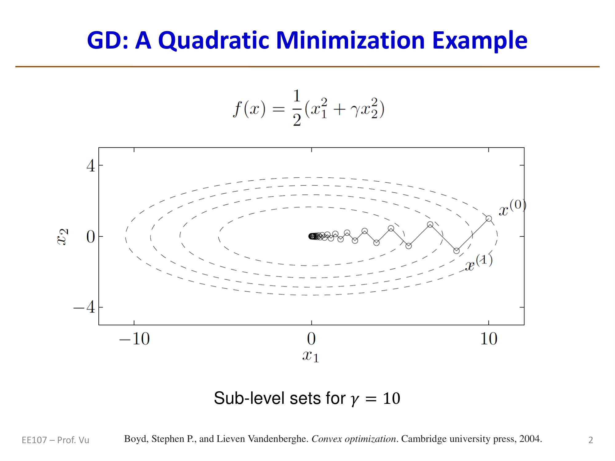
Convergence rate analysis:

• When \(\frac{1}{3} \leq \gamma \leq 3\): convergence is fast (condition number close to 1, contour lines are nearly circular)
• When \(\gamma \gg 1\) or \(\gamma \ll 1\): convergence is extremely slow (contour lines are highly elongated ellipses)
• GD exhibits approximately linear convergence (each step reduces the objective by a constant factor), with convergence rate depending on the Hessian condition number
• To reduce the distance by a factor of \(e^k\), GD requires approximately \(t \approx \frac{1}{2}k\kappa\) iterations

Key properties of GD:

• Computationally efficient: each step requires only vector multiplication and addition \(\theta^+ = \theta - \lambda \cdot \nabla J(\theta)\)
• Convergence rate is \(O(\kappa)\): the larger the condition number, the slower the convergence
• Momentum methods can improve convergence to \(O(\sqrt{\kappa})\); see the Optimizer notes for details

GD in Non-Convex Optimization

For a non-convex function \(J(\theta)\), solving \(\nabla J(\theta) = 0\) may yield:

• A local minimum \(\theta_1\)
• A local maximum \(\theta_2\)
• A global minimum \(\theta_3\)
• A saddle point \(\theta_4\) (a maximum in some directions, a minimum in others)

At all these points \(\nabla J(\theta) = 0\), but only the minima are what we seek. Therefore, in non-convex optimization, it is necessary to monitor whether \(J(\theta^{(k)})\) is consistently decreasing throughout the iteration process.

Convex Optimization

We have already mentioned that a zero gradient may occur at a saddle point, so a zero gradient alone does not guarantee that the function has reached an extremum. However, we all know that for a quadratic function like \(y = x^2\), its derivative \(y' = 2x\) is monotonically increasing. To the left of the zero-derivative point, the derivative is always negative (function decreasing); to the right, it is always positive (function increasing). In other words, the zero-derivative point must be a minimum. Note that on the derivative's coordinate plot, a negative derivative means the function decreases as we move to the right.

To generalize this intuition to multivariate functions, the concept of convex functions was introduced. For a function \(f(x)\), if for any \(x_1, x_2\) and \(0 < \alpha < 1\), the following holds:

\[ \alpha f(x_1) + (1 - \alpha)f(x_2) \geq f(\alpha x_1 + (1 - \alpha)x_2) \]

then \(f\) is a convex function.

In optimization algorithms (such as gradient descent), if the objective function is convex, we can guarantee that the function surface has no erratic "bumps" or "humps." The local optimum is the global optimum. In other words, as long as we keep following the gradient downhill, we will inevitably reach the unique lowest point without falling into other "small pits."

Convex optimization studies how to find the minimum of a convex function subject to specific constraints. In mathematics and engineering, convex optimization is considered a "gold standard" because it possesses an extremely attractive property: local optima are global optima.

Many traditional engineering and finance problems are inherently convex or can be perfectly reduced to convex functions. In these domains, convex optimization is a dominant tool. However, for deep learning problems, the objective function is almost always non-convex.

Although the global landscape of a neural network is generally non-convex, if we zoom into an extremely small region, any smooth curve looks like a tiny bowl. This is also a basic premise underlying optimizers discussed later — for instance, the Adam optimizer treats the local landscape as convex.

Of course, we must always keep saddle points in mind. Optimizers use momentum to skip past these saddle points where the gradient is zero at the center. Specifics are covered in the Optimizer section.

Stochastic Gradient Descent

Stochastic Gradient Descent (SGD) has its theoretical foundation in a paper titled "A Stochastic Approximation Method," proposed by Herbert Robbins and Sutton Monro in 1951.

SGD is a fast optimization algorithm whose core idea is "randomly sample a small portion, iterate quickly." It works as follows: unlike the standard method that examines all data before updating, SGD randomly samples a small batch (or even a single sample) of data each time to compute the gradient and immediately adjusts the model parameters. In GD, we need to pass through the entire training set to compute a single gradient and perform one parameter update (one step). If the dataset contains millions of examples, taking a single step would take an eternity. SGD is a clever improvement: each time it randomly grabs a small handful of data (a mini-batch), say 64 images, estimates the approximate gradient direction from that handful, and takes a step immediately.

The core update formula of SGD is:

\[ \theta := \theta - \eta \cdot \nabla_{\theta} J(\theta; x^{(i)}, y^{(i)}) \]

where:

• \(\theta\): represents the model parameters (the vector containing all weights and biases). Our goal is to find the optimal \(\theta\) through training.
• \(:=\) denotes the assignment operation.
• \(\eta\): eta, the learning rate, controlling the step size of each parameter update. A larger \(\eta\) means larger update magnitudes.
• \(\nabla_{\theta}\): the gradient. The gradient is a vector pointing in the direction of steepest increase of the loss function, which is why gradient descent adds a negative sign in front.
• \(J(\theta; x^{(i)}, y^{(i)})\): the loss function, measuring how poorly the model predicts on a single training sample \((x^{(i)}, y^{(i)})\). \(x^i\) is the feature of the \(i\)-th training sample, and \(y^i\) is its true label.

As can be seen, the update formula of SGD differs from traditional GD only in the batch size. Traditional gradient descent is also called Batch Gradient Descent (BGD), whose core idea is to use all training data to compute the gradient for each parameter update: \(\theta := \theta - \eta \cdot \nabla_{\theta} J(\theta)\). SGD's loss function targets only a single sample, making computation faster.

Advantages:

• Fast: low computational cost, especially well-suited for large-scale datasets. Extremely high parameter update frequency and fast training.
• Avoids local optima: the random "noise" in update directions helps escape suboptimal solutions in search of the global optimum.

Disadvantages:

• Unstable: the descent path oscillates and is not smooth. Each individual step may be somewhat inaccurate, but the overall trend is downward.
• May not converge: the algorithm may hover around the optimum rather than reaching it precisely.

In practice, mini-batch gradient descent (Mini-batch GD) is most commonly used — a compromise between SGD and full-batch gradient descent that balances speed and stability. From the purest definition of SGD, each parameter update uses only a single randomly selected training sample, such as:

• One row of tabular data
• One image and its label
• One sentence from an article, or one document from a collection

Since modern hardware — especially GPUs — excels at parallel data processing, in practice we typically use a mini-batch of samples (e.g., 32, 64, or 128) to compute the gradient. Beyond higher computational efficiency, using just 1 training sample can be very noisy and random, causing severe oscillation during training. Using the average gradient over a batch yields a more stable convergence process (closer to the true gradient). In deep learning discussions and papers, SGD generally refers to mini-batch gradient descent, not pure stochastic gradient descent.

Gradient Variance Analysis of SGD

SGD uses mini-batches to estimate the full gradient. Let the mini-batch size be \(m\). The SGD gradient estimate is:

\[ \hat{g} = \frac{1}{m} \sum_{i=1}^{m} \nabla_\theta L\!\left(f(x_i; \theta),\; y_i\right) \]

This estimate is an unbiased estimator of the full gradient: \(\mathbb{E}[\hat{g}] = \nabla_\theta J(\theta)\). However, its variance is inversely proportional to the batch size:

\[ \text{Var}[\hat{g}] = \frac{\sigma^2}{m} \]

where \(\sigma^2\) is the variance of the gradient from a single sample. This means:

• Larger batch: lower variance, more accurate gradient estimate, but higher computation cost per step
• Smaller batch: higher variance, more noise introduced, but higher update frequency

The advantage of SGD over full-batch GD is that full-batch GD requires \(O(N)\) computations for one update (where \(N\) is the total number of samples), while SGD only requires \(O(m)\). When \(m \ll N\), SGD can complete more parameter updates within the same computational budget, often reducing the loss more quickly.

Generalization Error and SGD

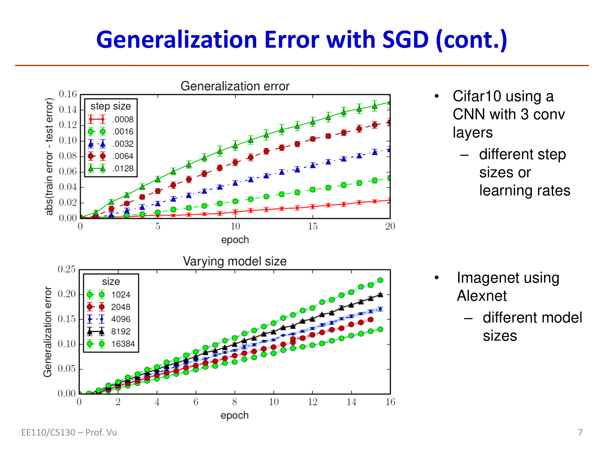
The stochasticity of SGD is not merely a computational convenience — it also provides an important generalization advantage. Hardt et al. (2016, Train faster, generalize better) proved from the perspective of algorithmic stability:

If SGD terminates within \(T\) steps, with each step using a mini-batch of size \(m\), then the generalization error of SGD satisfies:

\[\varepsilon_{gen} = |f(\theta) - g(\theta)| = O\!\left(\frac{T}{N}\right)\]

where \(f(\theta)\) is the true risk, \(g(\theta)\) is the empirical risk, and \(N\) is the training set size.

Important implications of this result:

• Early stopping has theoretical justification: fewer training steps \(T\) yield a smaller upper bound on generalization error
• SGD's noise serves as implicit regularization: compared to full-batch GD, SGD tends to converge to "flatter" minima (flat minima), which have better generalization performance. Intuitively, flat minima are insensitive to small parameter perturbations, so the model performs more consistently across training and test sets
• Large batches may harm generalization: excessively large batch sizes reduce gradient noise, potentially causing the model to converge to "sharp" minima, which actually degrades generalization performance

Gradient Explosion and Vanishing

When training deep networks (especially RNNs), gradients can grow or shrink exponentially with the number of layers, causing training failure. This problem was systematically analyzed by Pascanu et al. (2013, On the difficulty of training recurrent neural networks).

Mathematical Derivation in RNNs

Consider a simple RNN whose hidden state recurrence is:

\[ h_t = g(W_r^T h_{t-1} + W_x^T x_t + b) \]

where \(W_r\) is the recurrent weight matrix and \(g\) is the activation function. To compute the gradient of loss \(L\) with respect to parameters at early time steps, the chain rule propagates the gradient from time step \(t\) back to time step \(k\):

\[ \frac{\partial h_t}{\partial h_k} = \prod_{i=k+1}^{t} \frac{\partial h_i}{\partial h_{i-1}} = \prod_{i=k+1}^{t} \text{diag}\!\left(g'(z_i)\right) W_r^T \]

where \(z_i = W_r^T h_{i-1} + W_x^T x_i + b\) is the input to the activation function.

The key insight lies in the behavior of this chain product. Performing an eigenvalue decomposition on \(W_r^T\), let the spectral radius (the absolute value of the largest eigenvalue) be \(\rho = |\lambda_{\max}(W_r^T)|\):

• When \(\rho < 1\): \(\left\|\prod_{i=k+1}^{t} \text{diag}(g'(z_i)) W_r^T\right\| \to 0\), gradient exponentially decays → vanishes
• When \(\rho > 1\): \(\left\|\prod_{i=k+1}^{t} \text{diag}(g'(z_i)) W_r^T\right\| \to \infty\), gradient exponentially grows → explodes

More rigorously, Pascanu et al. proved:

\[ \left\|\frac{\partial h_t}{\partial h_k}\right\| \leq \left(\|W_r\| \cdot \gamma\right)^{t-k} \]

where \(\gamma = \max_i \|g'(z_i)\|\) is the upper bound of the activation function derivative (for Sigmoid, \(\gamma \leq \frac{1}{4}\); for Tanh, \(\gamma \leq 1\)). Therefore:

• If \(\|W_r\| \cdot \gamma < 1\): gradients necessarily vanish
• If \(\|W_r\| \cdot \gamma > 1\): gradients may explode (not necessarily — it depends on the specific \(g'(z_i)\) values)

Gradient Clipping

Gradient clipping is the most straightforward method for preventing gradient explosion (Pascanu et al., 2013). The idea is: when the gradient norm exceeds a threshold \(c\), scale it back to within the threshold:

\[ \hat{g} = \begin{cases} g & \text{if } \|g\| \leq c \\ \frac{c}{\|g\|} g & \text{if } \|g\| > c \end{cases} \]

This preserves the direction of the gradient while limiting only its magnitude. In PyTorch:

torch.nn.utils.clip_grad_norm_(model.parameters(), max_norm=1.0)

Strategies for Mitigating Gradient Vanishing

The gradient vanishing problem is more insidious because, unlike explosion, it does not produce obvious numerical anomalies. Common mitigation strategies include:

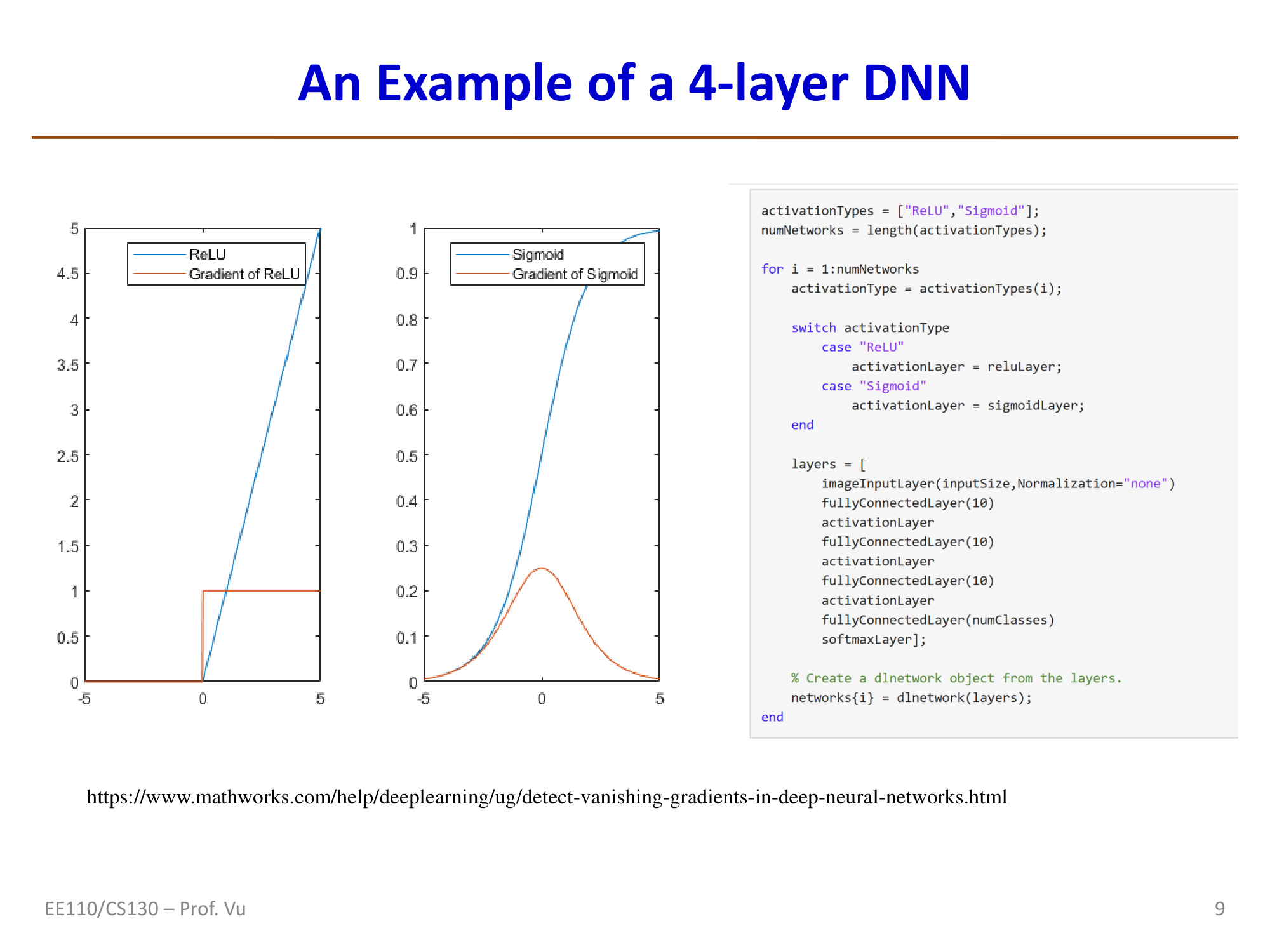
• ReLU activation function: \(g'(z) = 1\) (when \(z > 0\)), avoiding the problem of Sigmoid/Tanh derivatives being consistently less than 1
• Residual connections: \(h_\ell = F(h_{\ell-1}) + h_{\ell-1}\), providing a direct gradient pathway
• LSTM/GRU gating mechanisms: controlling information flow through forget gates and input gates to prevent gradient vanishing in long-range dependencies
• Proper initialization (e.g., Xavier, Kaiming initialization): maintaining stable variance of activations across layers
• Normalization techniques (e.g., BatchNorm, LayerNorm): stabilizing the input distribution at each layer

---

评论