LSTM
Questions to consider:
- What roles do the "cell state" and "hidden state" play in LSTM, respectively? Why are two information pathways needed?
- What problem does each of the three gates (forget, input, output) solve? What would happen if one were removed?
- Why does LSTM mitigate vanishing gradients? Can it completely prevent exploding gradients?
Background and Motivation
The Long-Term Dependency Problem in RNNs
As discussed in the RNN fundamentals notes, a vanilla RNN passes information between time steps through the hidden state \(h_t\). However, this single information pathway has a serious flaw:
At every time step, information must pass through \(\tanh\) (which compresses values to \([-1,1]\)) and a matrix multiplication \(W_{hh}\). During BPTT (Backpropagation Through Time), the gradient involves a chain of multiplications:
Since \(\tanh' \in (0, 1]\), this product decays exponentially as the time span \(T - k\) grows, causing the gradient at earlier time steps to approach zero — this is the vanishing gradient problem.
Intuitive understanding: Imagine a game of telephone where every person "compresses" the message before passing it on. After 50 people, the original message is almost entirely lost. Vanilla RNNs behave the same way — they cannot retain information from dozens of steps ago.
The Core Idea Behind LSTM
Long Short-Term Memory (LSTM) was introduced by Hochreiter & Schmidhuber in 1997. The central idea is:
Core Design Principle
In addition to the hidden state \(h_t\), introduce a separate cell state \(C_t\) that acts as an "information highway." Information travels along this highway through element-wise multiplication and addition (linear operations) only, without passing through squashing activation functions. This allows gradients to propagate over long distances with minimal loss.
Three gating mechanisms are introduced to precisely control the flow of information:
- Forget Gate: decides what old information to discard
- Input Gate: decides what new information to write
- Output Gate: decides what information to expose as output
All three gates use the sigmoid function to output values between 0 and 1, acting as "soft switches."
LSTM Architecture in Detail
Full Architecture Overview
The figure below shows the complete internal structure of an LSTM cell (source: GeeksForGeeks):
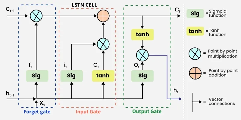
Symbol legend:
| Symbol | Meaning |
|---|---|
| Sig | Sigmoid activation function, output \(\in (0, 1)\) |
| tanh | Tanh activation function, output \(\in (-1, 1)\) |
| \(\otimes\) | Element-wise multiplication (Hadamard product) |
| \(\oplus\) | Element-wise addition |
| Straight arrows | Vector concatenation and data flow |
Inputs and outputs of an LSTM cell:
- Inputs: current input \(x_t\), previous hidden state \(h_{t-1}\), previous cell state \(C_{t-1}\)
- Outputs: current hidden state \(h_t\), current cell state \(C_t\)
Note that LSTM has two information pathways:
- Cell state \(C_t\) (horizontal line at the top): the long-term memory channel, where information flows via linear operations so that gradients can propagate over long distances
- Hidden state \(h_t\) (horizontal line at the bottom): the short-term memory channel, which is exposed as the external output
Step 1: Forget Gate — "What old memories to discard?"
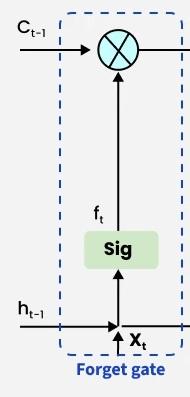
The forget gate decides how much old information to discard from the cell state. It examines the previous hidden state \(h_{t-1}\) and the current input \(x_t\), then outputs a vector with values between 0 and 1:
where \([h_{t-1}, x_t]\) denotes the concatenation of the two vectors.
Each element of \(f_t\) controls how much of the corresponding dimension of \(C_{t-1}\) is retained:
- \(f_t[i] \approx 1\): fully retain the memory in dimension \(i\) ("remember")
- \(f_t[i] \approx 0\): fully erase the memory in dimension \(i\) ("forget")
Example: In a language model, when a new subject "she" appears, the forget gate may decide to erase the gender information associated with the previous subject "he."
Step 2: Input Gate — "What new memories to write?"
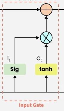
The input gate decides what new information to write into the cell state. This involves two sub-steps:
Sub-step A: Decide "how much to write"
The sigmoid output (0 to 1) controls the write intensity for each dimension.
Sub-step B: Generate "what to write"
The tanh output produces a candidate value vector in \([-1, 1]\), representing the potential new information to be written.
The actual new information written is \(i_t \odot \tilde{C}_t\) (element-wise multiplication) — that is, \(i_t\) filters \(\tilde{C}_t\).
Step 3: Update the Cell State — The Core Equation
With the outputs of the forget gate and the input gate, the cell state is now updated:
This is the most critical equation in LSTM. Its meaning is highly intuitive:
Note that this involves only element-wise multiplication and addition — no matrix multiplication and no squashing activation functions. This "highway" allows information and gradients to travel over long distances, which is the key to how LSTM addresses the vanishing gradient problem.
Step 4: Output Gate — "What to output?"
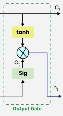
The output gate decides what information from the current cell state to expose as the hidden state:
The cell state is first mapped to \([-1, 1]\) through \(\tanh\), then filtered by the output gate. The resulting \(h_t\) is the hidden state exposed to the outside world, and it serves three purposes:
- Passed to the LSTM cell at the next time step
- Used as the output at the current time step (in many-to-many tasks)
- Used as the final output (at the last step of many-to-one tasks)
Formula Summary
| Step | Formula | Activation | Purpose |
|---|---|---|---|
| Forget gate | \(f_t = \sigma(W_f \cdot [h_{t-1}, x_t] + b_f)\) | Sigmoid | Controls how much old memory to retain |
| Input gate | \(i_t = \sigma(W_i \cdot [h_{t-1}, x_t] + b_i)\) | Sigmoid | Controls the write intensity of new information |
| Candidate value | \(\tilde{C}_t = \tanh(W_C \cdot [h_{t-1}, x_t] + b_C)\) | Tanh | Generates candidate new information |
| Cell update | \(C_t = f_t \odot C_{t-1} + i_t \odot \tilde{C}_t\) | None | Merges old memory with new information |
| Output gate | \(o_t = \sigma(W_o \cdot [h_{t-1}, x_t] + b_o)\) | Sigmoid | Controls what information to output |
| Hidden state | \(h_t = o_t \odot \tanh(C_t)\) | Tanh | Produces the output for the current time step |
Parameter count: Four weight matrices \(W_f, W_i, W_C, W_o \in \mathbb{R}^{d_h \times (d_h + d)}\) and four bias vectors. The total parameter count is approximately \(4 \times d_h \times (d_h + d)\), which is 4 times that of a vanilla RNN.
Forward Pass: A Complete Numerical Example
Setup: \(d = 4\) (input dimension), \(d_h = 3\) (hidden state dimension).
Processing the sequence "我 喜欢 猫" (I like cats), starting with the first word "我" (I):
Inputs: \(x_1 = [0.21, -0.45, 0.73, 0.12]\), \(h_0 = [0, 0, 0]\), \(C_0 = [0, 0, 0]\)
Step 1: Concatenation
Step 2: Four matrix multiplications (one for each gate)
Each gate computes: 7-dimensional input \(\rightarrow\) matrix multiplication with \(W \in \mathbb{R}^{3 \times 7}\) \(\rightarrow\) add bias \(\rightarrow\) activation function \(\rightarrow\) 3-dimensional output.
Step 3: Update the cell state
Step 4: Compute the hidden state
When processing "喜欢" (like), \(h_1\) and \(C_1\) are fed as inputs and the exact same procedure is repeated.
Why Does LSTM Solve the Vanishing Gradient Problem?
The key lies in the additive structure of the cell state update:
When the gradient is backpropagated along the cell state:
Comparison with vanilla RNN:
| Vanilla RNN | LSTM (along cell state) | |
|---|---|---|
| Gradient propagation | \(\frac{\partial h_t}{\partial h_{t-1}} = W_{hh}^T \cdot \text{diag}(\tanh')\) | \(\frac{\partial C_t}{\partial C_{t-1}} = f_t\) |
| Chain product | \(\prod W_{hh}^T \cdot \text{diag}(\tanh')\) \(\rightarrow\) uncontrollable | \(\prod f_t\) \(\rightarrow\) learnable and controllable |
| Issue | Eigenvalues of \(W_{hh}\) determine the gradient's fate | \(f_t\) is a sigmoid output and can learn to be close to 1 |
When the model learns that certain information needs to be retained over the long term, the forget gate outputs values close to 1 (\(f_t \approx 1\)), allowing the gradient to pass through arbitrarily many time steps with minimal loss. This is like cruising on a highway, while a vanilla RNN is like traveling a back road with a toll booth every few meters.
LSTM does not completely prevent exploding gradients
LSTM mitigates vanishing gradients through its additive structure, but exploding gradients can still occur (especially when forget gates are close to 1 and gradients accumulate across many time steps). In practice, gradient clipping is needed to prevent gradient explosions.
Comparison with GRU
GRU (Gated Recurrent Unit, Cho et al., 2014) is a simplified variant of LSTM that merges the forget and input gates into a single update gate and removes the separate cell state. See the GRU notes for details.
| LSTM | GRU | |
|---|---|---|
| Number of gates | 3 (forget, input, output) | 2 (update, reset) |
| States | Two: \(h_t\) and \(C_t\) | One: \(h_t\) only |
| Parameter count | \(4 d_h(d_h + d)\) | \(3 d_h(d_h + d)\) (~25% fewer) |
| Performance | Slightly better on very long sequences | Comparable on most tasks |
| Training speed | Slower | Faster |
In practice, the difference between the two is small. If the dataset is small or the sequences are not too long, GRU may be more suitable; if sequences are very long and computational resources are ample, LSTM is generally the safer choice.
Practical Applications
Before the advent of the Transformer (pre-2017), LSTM was the dominant deep learning approach for sequential data. Typical applications include:
- Language modeling and machine translation: The predecessors of the GPT series were LSTM-based language models
- Speech recognition: Converting speech signal sequences into text
- Time series forecasting: Stock price prediction, weather forecasting, etc. — LSTM excels at capturing long-period patterns (e.g., seasonal trends)
- Anomaly detection: Identifying anomalous patterns in time series data
- Video analysis: Combining CNN-extracted frame features with LSTM for temporal modeling
Practical Tips
Hyperparameter Selection
| Parameter | Typical Range | Notes |
|---|---|---|
| Hidden state dimension \(d_h\) | 128 -- 512 | Larger for more complex tasks, but too large risks overfitting |
| Number of layers | 1 -- 3 | Diminishing returns beyond 3 layers; use residual connections |
| Dropout | 0.2 -- 0.5 | Applied between layers, not between time steps |
| Learning rate | 1e-3 -- 1e-2 | Typically 1e-3 with the Adam optimizer |
| Gradient clipping | 1.0 -- 5.0 | Prevents gradient explosion |
Common Techniques
- Initialize forget gate bias to a positive value (e.g., \(b_f = 1\)): This biases the model toward "remembering" rather than "forgetting" at the start, which improves training stability
- Use bidirectional LSTM: Unless the task involves generation, BiLSTM almost always outperforms unidirectional LSTM
- Last step vs. mean pooling: For tasks like sentiment analysis, averaging the hidden states across all time steps (mean pooling) can sometimes outperform using only the last time step
- Pretrained word embeddings: Initializing the embedding layer with Word2Vec or GloVe converges faster than random initialization
Historical Significance of LSTM
| Period | Status |
|---|---|
| 1997--2013 | Largely overlooked after publication (insufficient compute and data) |
| 2013--2017 | Rose to become the dominant architecture for sequence modeling with the deep learning boom, ruling NLP, speech, and time series |
| 2017--present | Gradually superseded by the Transformer (almost entirely replaced in NLP), but still used for small-data regimes, long time series, and edge devices |
LSTM's greatest contribution is not just the architecture itself, but the pioneering gating mechanism concept — an idea that later influenced GRU, Highway Networks, residual connections, and various gating variants within the Transformer.
Next up: \(\rightarrow\) Seq2Seq (combining two LSTMs into an encoder-decoder framework to solve sequence-to-sequence problems)