Theory of Computation: Automata Theory

These notes follow the classic textbook Introduction to the Theory of Computation, 3rd/4th Edition as the primary reference, covering only the most essential content in a concise manner. Since my main interests lie in artificial intelligence and robotics, this entire notebook is organized as a single page rather than being broken into individual pages per chapter as with my reinforcement learning or deep learning notes.

This book and course guide us through a fundamental question:

What are the fundamental capabilities and limitations of computers?

What are the fundamental capabilities and limitations of computers?

It is difficult to perform mathematical analysis directly on a computational problem. Therefore, we call a set of strings a language, transform a problem into a language, and then apply rigorous mathematical tools to analyze it. In other words, any "yes/no" computational problem can be viewed as a language recognition problem.

From this perspective, the theory of computation has three major themes, all of which study how to work with languages:

1. Automata (Automata Theory) — Ch.1 - Ch.2

Automata theory studies what kinds of machines can recognize what kinds of languages:

What languages can the simplest finite automata recognize? — Regular languages
What languages can the more complex pushdown automata recognize? — Context-free languages
What languages can the most powerful Turing machines recognize? — All computable languages

2. Computability (Computability Theory) — Ch.3 - Ch.5

Computability theory studies which languages a computer can recognize (i.e., problems a computer can solve) and which it cannot. If we can find a language for which no algorithm (Turing machine) can ever be designed to perfectly determine whether a string belongs to it, then that language is undecidable (i.e., the problem is unsolvable by computer). For example, the language corresponding to the "halting problem" is undecidable.

3. Complexity (Computational Complexity Theory) — Ch.6 - Ch.7

Computational complexity theory studies how many resources are needed to recognize a language — that is, among solvable problems, which are easy and which are hard to solve. In the famous P vs NP problem, both P and NP are collections of languages. P-class languages are problems that can be solved quickly (in polynomial time). NP-class languages are problems whose solutions, once guessed, can be quickly verified. The P vs NP problem essentially asks whether these two sets of languages are equal.

The most direct application of computational complexity theory is cryptography, where security is achieved by identifying computationally hard problems.

Ch.0 Foundations of Discrete Mathematics

A solid grounding in discrete mathematics is generally required before studying the theory of computation. Here we briefly review the main topics, focusing not on a comprehensive treatment of discrete mathematics but rather on the foundations needed for computation theory. The examples in this section will accordingly emphasize computation-theory-related content.

The most commonly used mathematical tools in computation theory almost all come from discrete mathematics, including:

Set
Union, Intersection, Complement
Sequence
Tuple
Cartesian Product (Cross Product)
Function
Mapping
Graph
Undirected Graph, Directed Graph
String, Lexicographic Order

Boolean Logic:

AND ∧
OR ∨
NOT ¬
Exclusive OR ⊕ (only 1⊕0 equals 0)
Equality ↔
Implication → (only 1→0 equals 0)

Definitions, theorems, and proofs:

Defination
Mathematical Statement
Proof
Theorem
Lemma
Corollary
Counterexample

Proposition notation:

⟺ iff, if and only if
for P⟺Q:
- forward direction: P⟹Q
- reverse direction: Q⟹P

Types of proofs:

Proof by Construction
Proof by Contradiction
Proof by Induction
- Basis
- Induction Step

0.1 Logic and Proof Methods

Proof by Induction

The method of proof by induction proceeds from small to large: first prove the base case (e.g., the empty string or the shortest string), then assume the proposition holds for length $k$, and show it also holds for $k+1$. The entire logical chain relies on the inductive hypothesis, which builds up by increasing length.

Induction is very rigorous and well suited for scenarios such as:

When the language or property is closely tied to string length, e.g., "strings of any length satisfy a certain structure."
Proving recursively defined languages, such as languages generated by regular expressions or recursive grammars.
Properties involving incremental growth, e.g., "no matter how many characters have been read, the DFA maintains a certain invariant."

Example:

1758719123259

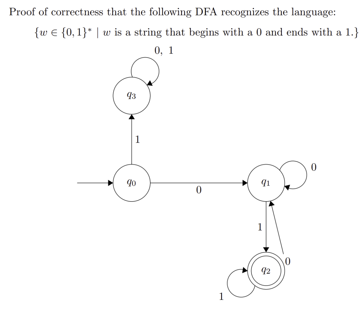
Proof:

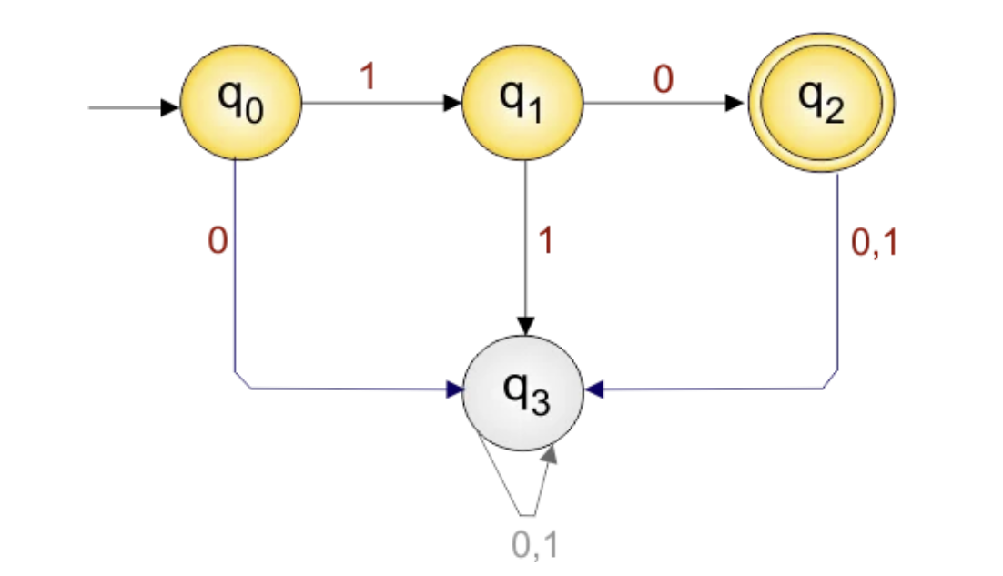
This DFA recognizes the language by proof of induction on the length of the input string such that the DFA always ends in the correct state according to the last symbol and the requirement that the string starts with 0.

Base Case:

If w is a single 0, the DFA moves from q₀ to q₁. The DFA does not accept this string because it doesn't begin with a 0 AND end with a 1.
If w is a single 1, the DFA moves from q₀ to q₃. The DFA does not accept this string and will never accept because it doesn't begin with a 0.
If w is the empty string, the DFA will immediately reject because it doesn't begin with a 0 or end with a 1.

Inductive Steps:

Suppose the DFA is in the correct state after reading a string of length k and let w be a string that begins with a 0 and ends with a 1 of length k + 1.

If w began with a 1, the DFA transitioned to q₁ and will never accept due to an infinite loop.
Otherwise, if w began with a 0, the DFA can either be in q₁ or q₂ after reading in k characters.

Now there are two cases:

The last character of w is a 0
The last character of w is a 1

In the first case, if the last character of w is a 0, regardless of whether the DFA is in q₁ or q₂, the DFA will end in q₁ and reject.

In the second case, if the last character of w is a 1, regardless of whether the DFA is in q₁ or q₂, the DFA will end in q₂ and accept.

We know that the DFA only accepts a string iff (if and only if) it ends in q₂ and by the invariant, q₂ means the string starts with 0 and ends with 1.

Conversely, if the string does not begin with 0, the DFA will go into an infinite loop in q₃ and reject.

And if the string does not end with 1, the DFA will end in q₁ and reject.

Proof by Construction

Proof by construction, also called case analysis, is more intuitive and straightforward than induction. However, construction obviously cannot classify languages involving arbitrary length or recursive structure (i.e., it cannot handle infinitely many cases).

Construction is well suited for scenarios such as:

When the language property is relatively local and can be fully covered by a finite number of cases.
When the DFA design is clearly based on several distinct patterns, so that analyzing each case directly yields the conclusion.

Example:

1758719123259

Proof:

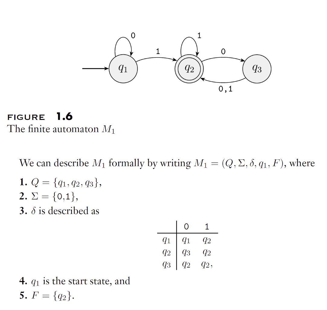
This DFA recognizes the language by proof of construction by breaking up how the DFA handles strings in different cases.

For any string w, w will either be one of the following:

w begins with a 0 and ends with a 1
w begins with a 0 and doesn't end with a 1
w doesn't begin with a 0 and ends with a 1
w doesn't begin with a 0 and doesn't end with a 1

In case 1, the DFA must transition to q₁ since w begins with a 0 and it must end up in q₂ because regardless of whether the DFA is in q₁ or q₂ before the last character is read, it will always end in q₂. Therefore, strings in this case will always get accepted.

In case 2, the DFA must transition to q₁ since w begins with a 0 and it must end up in q₁ because regardless of whether the DFA is in q₁ or q₃ before the last character is read, it will always end in q₁. Therefore, strings in this case will always be rejected.

In case 3 and 4 (which can be combined), the DFA must transition to q₃ since w begins with a 1 and will remain in q₃ as the state loops on all inputs. Therefore, strings in this case will always be rejected.

From the above cases, the only strings that can be accepted by this DFA are those that begin with a 0 and end with a 1 (case 1). All other cases result in the string being rejected. Therefore, the DFA recognizes the above language.

Proof by Contradiction

(To be added)

0.2 Mathematical Concepts and Terminology

Sets, sequences, tuples, and Cartesian products

Functions, mappings, and relations

Equivalence relations, partial orders

Injections, surjections, bijections

Invertibility, function composition

Combinatorics and counting principles

Permutations and combinations
Pigeonhole principle
Basic probability

Graph theory basics

Graphs and subgraphs, trees
Paths, connectivity
Euler paths, Hamiltonian paths

Number theory basics

Divisibility, modular arithmetic
Primes and congruences
Helpful for cryptography and computability

Boolean logic (Section 0.2.6 of the textbook)

Ch.1 Regular Languages

1.1 Strings and Languages

Strings are one of the fundamental building blocks of computer science. Depending on the application, strings can be defined over a wide variety of alphabets. By convention, an alphabet is defined as any nonempty finite set. The members of an alphabet are called the symbols of that alphabet. Alphabets are typically denoted by the uppercase Greek letters $\Sigma$ (Sigma) and $\Gamma$ (Gamma), which represent both the alphabet itself and the printable characters of its symbols. Here are a few examples of alphabets:

\[ \Sigma_1 = \{0,1\} \]

\[ \Sigma_2 = \{a, b, c, d, e, f, g, h, i, j, k, l, m, n, o, p, q, r, s, t, u, v, w, x, y, z\} \]

\[ \Gamma = \{0,1,x,y,z\} \]

A string over an alphabet is a finite sequence of symbols from that alphabet, usually written as symbols placed one after another without separating commas. Let $\Sigma_1=\{0,1\}$; then $01001$ is a string over $\Sigma_1$. Let $\Sigma_2=\{a,b,c,\cdots,z\}$; then abracadabra is a string over $\Sigma_2$.

Let $w$ be a string over $\Sigma$. The length of $w$ is the number of symbols it contains, denoted $|w|$. A string of length zero is called the empty string and is written as $\epsilon$. The empty string plays a role analogous to zero in the ring of integers. If $w$ has length $n$, it can be written as:

\[ w = w_1 w_2 \cdots w_n, \quad \text{这里每个 } w_i \in \Sigma. \]

Its reverse is the string obtained by writing $w$ in the opposite order, denoted $w^R$:

\[ w^R = w_n w_{n-1} \cdots w_1. \]

If the string $x$ appears consecutively within $w$, then $x$ is called a substring of $w$. For example, cad is a substring of abracadabra.

Let $x$ be a string of length $m$ and $y$ a string of length $n$. The concatenation of $x$ and $y$ is the string obtained by appending $y$ to the end of $x$, denoted $xy$:

\[ xy = x_1 \cdots x_m y_1 \cdots y_n. \]

Superscript notation can be used to denote a string concatenated with itself multiple times; for example, $x^k$ means:

\[ \underbrace{xx\cdots x}_{k \text{次}}. \]

Lexicographic order is the familiar dictionary ordering. Typically, we use shortlex order (also called string order), which places shorter strings before longer ones on top of lexicographic order. For example, the string order of all strings over the alphabet $\{0,1\}$ is:

\[ (\epsilon, 0, 1, 00, 01, 10, 11, 000, \cdots) \]

String $x$ is a prefix of string $y$ if there exists a string $z$ such that $y = xz$. If and only if $x \neq y$, then $x$ is called a proper prefix of $y$.

A set of strings is called a language. If no member of a language is a prefix of any other member, then the language is prefix-free.

1.2 Finite State Machines

Real-world computers are too complex, so we begin by studying simpler and more abstract models. We use a computational model to abstract a computer, retaining only the core features we care about.

We focus on states and transitions between them, without considering complex memory or hardware. This kind of model is therefore called a finite state machine (FSM), also known as a finite automaton (FA).

Note that a finite automaton has only finitely many states and no additional storage, so it is not the kind of computer we use today. Modern computers more closely approximate Turing machines (which technically have infinite storage, but today's computers have such vast storage capacity that they can be considered approximate Turing machines) rather than finite state machines.

Of course, many real-world systems are effectively finite state machines, such as traffic lights, vending machines, and remote controls.

In general, we primarily focus on DFA (Deterministic Finite Automaton), i.e., deterministic finite state machines. The core distinction between DFA and NFA is: for each state, a DFA has exactly one transition for every valid symbol in the alphabet, whereas an NFA may have multiple (or zero) transitions.

A finite automaton FA can be defined as a 5-tuple:

\[ (Q, \Sigma, \delta, q_{0}, F) \]

where

$Q$ is a finite set called the states
$\Sigma$ is a finite set called the alphabet
$\delta : Q \times \Sigma \to Q$ is the transition function
$q_{0} \in Q$ is the start state
$F \subseteq Q$ is the set of accept states

An FA must have a start state, but in special cases the set of accept states may be empty.

The above 5-tuple is also called the formal definition of a finite automaton (FA). This 5-tuple is "formal" because it uses precise mathematical language (sets, functions, etc.) to describe an automaton with no ambiguity whatsoever. It precisely defines:

What states exist (Q)
What input symbols are accepted (Σ)
How to transition from one state to another (δ)
Which state to start from (q0)
Which states are final success states (F)

Any finite automaton, no matter how complex, can be unambiguously described by such a 5-tuple. This is the essence of a "formal definition."

When drawing a DFA, we use an arrow with no source to indicate the start state, and a double circle to represent an accept state. Accept states need not exist and there may be more than one. Below is an example of a state transition diagram:

1758724039765

If A is the set of strings that machine M accepts, we say: A is the language of machine M, and write:

\[ L(M) = A \]

We say that M recognizes A, or M accepts A. An FA machine may accept several strings, but it always recognizes exactly one language.

We can describe a DFA using a concise description:

Set notation
Regular expression
Natural language description

1758724348162

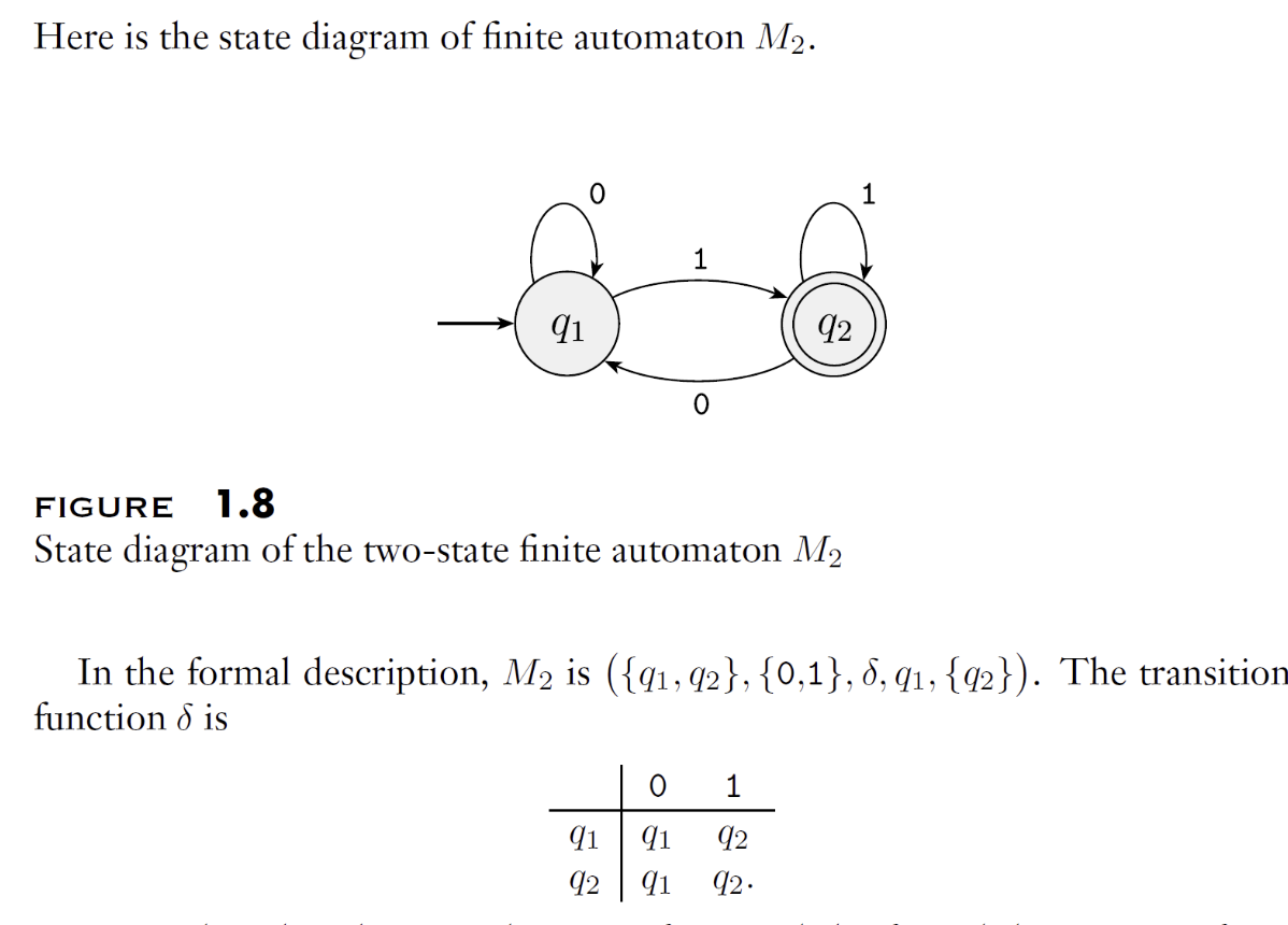
Taking the above diagram as an example, we can describe it in natural language:

M2 accepts exactly the set of binary strings that end with a 1.

Or in set notation:

\[ L(M_2) = \{ w \mid w \text{ ends in a } 1 \} \]

Or as a regular expression:

\[ L(M_2) = (0 + 1) * 1 \]

All three are concise descriptions.

Example 1: Identify the state transition diagram and describe the language of the DFA:

1758724847567

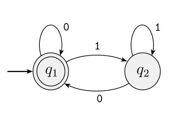
We can draw a state table or trace the transitions by substitution. We can see that upon receiving a 0, the machine transitions to q1; otherwise it transitions to q2. Since q1 is the accept state, this DFA (or machine) accepts strings ending in 0. That is:

\[ L(M) = \{\, w \mid w \text{ is the empty string } \varepsilon \text{ or ends in a } 0 \,\}. \]

Example 2: Identify the language recognized by the following DFA:

1758725025103

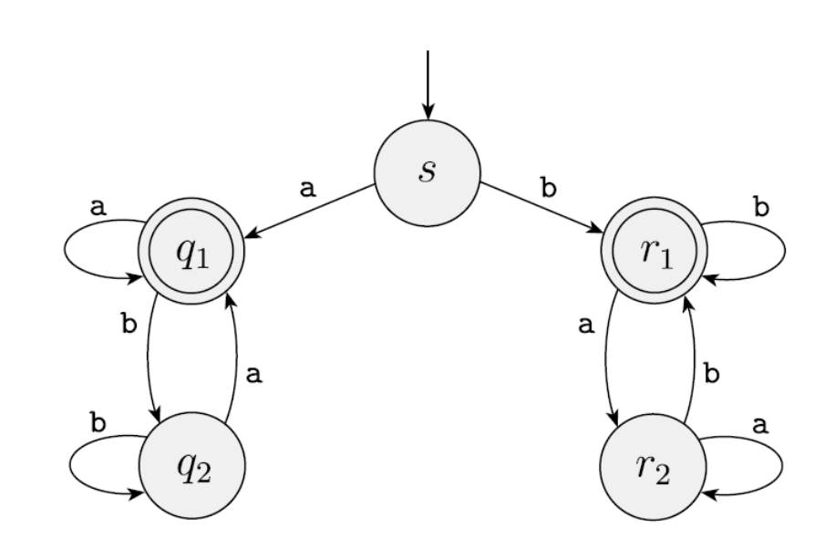
In this diagram, once a symbol is received, the machine goes to either q1 or r1, with no way to return to s. So this machine "remembers" the first symbol. If the machine ultimately accepts on an 'a', the first character was 'a'; if it accepts on a 'b', the first character was 'b'. More precisely, this machine accepts strings whose first and last symbols are the same:

\[ L(M) = \{\, w \mid w \text{ starts and ends with the same symbol} \,\} \]

Example 3: Identify the language recognized by the following DFA:

1758725231656

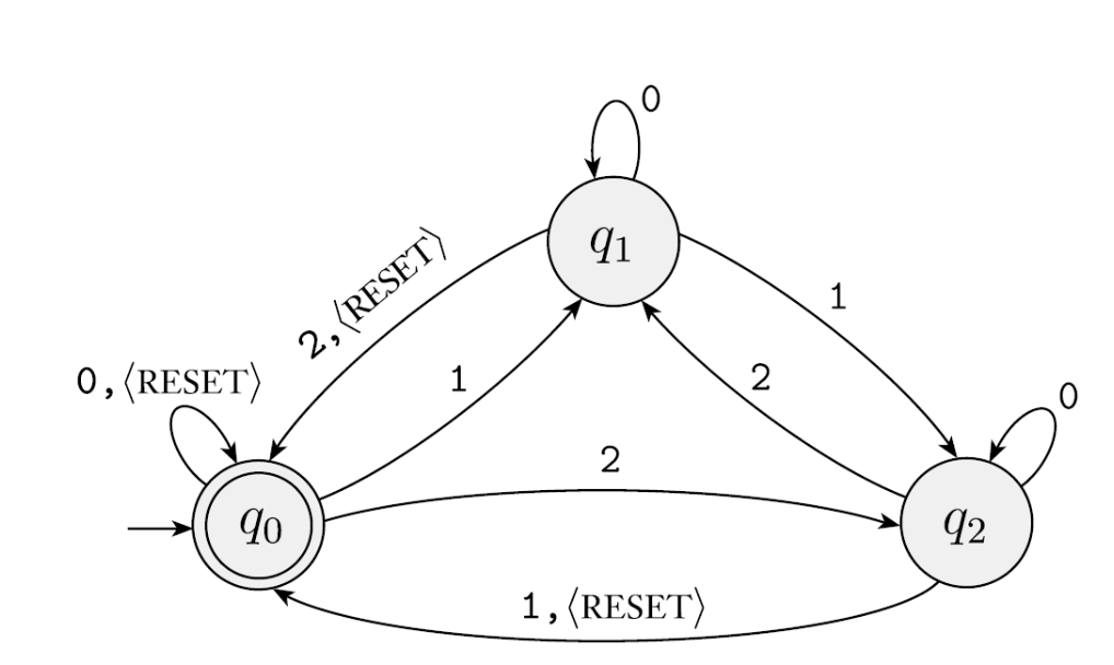
This machine has an additional <RESET> special symbol. The DFA starts at q0: if the input is 0 it accepts, if 1 it goes to q1, if 2 it goes to q2. At q1, if the input is 2 it returns to q0 and accepts; at q2, if the input is 1 it returns to q0... Upon careful inspection, this is essentially a modular arithmetic FA. The RESET symbol pauses the current modular computation and starts a new one.

We can generalize this DFA for modular arithmetic with any modulus, yielding the following machine:

For each $i \geq 1$ let $A_i$ be the language of all strings where the sum of the numbers is a multiple of $i$, except that the sum is reset to $0$ whenever the symbol $\langle \text{RESET} \rangle$ appears.

For each $A_i$ we give a finite automaton $B_i$, recognizing $A_i$. We describe the machine $B_i$ formally as follows:

\[ B_i = (Q_i, \Sigma, \delta_i, q_0, \{ q_0 \}), \]

where $Q_i$ is the set of $i$ states $\{ q_0, q_1, q_2, \dots, q_{i-1} \}$, and we design the transition function $\delta_i$ so that for each $j$, if $B_i$ is in $q_j$, the running sum is $j \pmod{i}$.

For each $q_j$ let:

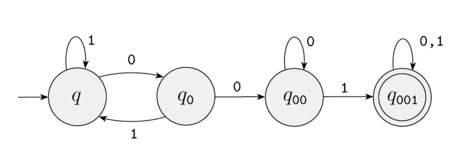
\[ \begin{aligned} \delta_i(q_j, 0) &= q_j, \\ \delta_i(q_j, 1) &= q_k, \quad \text{where } k = j+1 \pmod{i}, \\ \delta_i(q_j, 2) &= q_k, \quad \text{where } k = j+2 \pmod{i}, \\ \delta_i(q_j, \langle \text{RESET} \rangle) &= q_0. \end{aligned} \]

Example 4: Design a DFA that recognizes "binary strings containing at least one occurrence of the substring 001."

Solution approach:

Ignore all 1s
Once a 0 is seen, remember it as a potential first 0 of 001
If another 0 follows, remember it as a potential 00 of 001
If yet another 0 follows, remain in the 00 state
In the 00 state, seeing a 1 means 001 has been found — accept

1758725603425

Example 5: w accepts only the string "01"

1765786036155

1.3 Formal Definition

In the previous section, we introduced the 5-tuple formal definition and concise description methods. As mentioned above, in the theory of computation, a set of strings is called a "language," and this set may contain finitely or infinitely many strings.

Distinguish between alphabet and language:

An alphabet is a finite set of characters
A language is a set of strings, each being a finite sequence of characters from the alphabet

For example:

\[ L_{1} = \{\, \text{"cat"}, \text{"dog"}, \text{"fish"} \,\} \quad (\text{finite set}) \]

\[ L_{2} = \{\, \text{all strings ending with "ab"} \,\} \quad (\text{infinite set, e.g., "ab", "aab", "bab", }\dots) \]

When an automaton M can produce an "Accept" or "Reject" conclusion for every string w passed to it, we say:

\[ A = \{\, w \mid M \ \text{accepts } w \,\}. \]

This statement has two implications:

Every string M accepts is in language A
Every string M rejects is not in language A

Thus, automaton M serves as a perfect, precise "definition" or "rule" for language A. If a language can be associated with an FA that recognizes it in the manner described above, then we say it is a regular language. Conversely, if no such FA exists for a language, then it is not a regular language.

For example:

All binary strings ending in 1: An FA only needs to check whether the last character is 1 — this is a regular language.
All strings containing 007: We can design a few states to track whether consecutive 007 has appeared — this is a regular language.
All strings consisting of $n$ 0s followed by $n$ 1s: Since an FA has no memory, no FA can be designed to recognize this language — it is not a regular language.

1.4 Regular Operations

Closure Properties

Closure is a mathematical concept describing the relationship between a set and an operation. Its main idea is: if performing a certain operation on members of a set always produces a result that is still in the set, then the set is closed under that operation.

For example:

Addition is closed over the integers.
Division is not closed over the integers, since dividing two integers may yield a non-integer.
Addition is not closed over the odd numbers (odd + odd = even).
Strings are closed under concatenation.
The set of Boolean values is closed under AND.

Closure is a testing tool that describes whether a set is self-sufficient under a given operation. In the theory of computation, "regular languages are closed under regular operations" is a core theorem. This theorem is the theoretical cornerstone for building regular expressions, compilers, and other advanced tools.

Union

And the closure property of union.

Let A and B be two languages. The union operation is:

\[ A \cup B = \{ x \mid x \in A \;\text{or}\; x \in B \} \]

Concatenation

And the proof of the closure property of concatenation.

Let A and B be two languages. The concatenation operation is:

\[ A \circ B = \{ xy \mid x \in A \;\text{and}\; y \in B \} \]

Star

And the proof of the closure property of the star operation.

Let A and B be two languages. The star operation is:

\[ A^* = \{ x_1 x_2 \cdots x_k \mid k \geq 0 \;\text{and each } x_i \in A \} \]

1.5 Regular Expressions

A regular expression is an expression that uses symbols representing union, concatenation, and star to combine symbols representing the most basic languages (such as {a}, {ε}). We previously stated that a language recognizable by an FA is a regular language. After learning the regular operation symbols, we now have a new criterion: a language that can be expressed by a regular expression is a regular language.

In terms of descriptive power, regular expressions and DFAs are equivalent. In other words, every DFA can be described by a regular expression. Any language recognizable by a DFA can be described by some regular expression. Conversely, any language described by a regular expression can be recognized by some DFA.

This is not merely a coincidence but is guaranteed by a famous theorem — Kleene's Theorem. This theorem reveals a deep equivalence:

Regular Expressions ⇔ Finite Automata

Specifically, the following three ways of describing languages are completely equivalent in expressive power:

Regular Expression
Nondeterministic Finite Automaton (NFA)
Deterministic Finite Automaton (DFA)

They can describe one and only one class of languages, known as "Regular Languages".

This equivalence means we have explicit algorithms to convert between these forms:

Regular Expression → NFA: We can use Thompson's construction to convert any regular expression into an equivalent NFA.
NFA → DFA: We can use the subset construction to convert any NFA into an equivalent DFA.
DFA → Regular Expression: Algorithms such as the State Elimination Method or Brzozowski's Algebraic Method can convert any DFA into an equivalent regular expression.

To summarize the preceding sections:

First, we learned what regular languages are: languages recognizable by FAs are regular languages.
Then we learned three regular operation symbols: union, concatenation, and star.
Next, we learned that regular operations satisfy the closure property.
Finally, we elevated this to: languages expressible by regular operations are regular languages.

In Ch.1 Regular Languages, we learned that the following are mutually equivalent:

Finite Automata: DFA/NFA
Regular Expressions
Regular Grammar
5-Tuple

Regular languages are closed under the following main operations:

Union: $L_{1} \cup L_{2}$
Concatenation: $L_{1} \cdot L_{2}$
Kleene Star: $L_{1}^{*}$
Intersection: $L_{1} \cap L_{2}$
Complement: \overline{$L_{1}$}
Difference: $L_{1} - L_{2}$

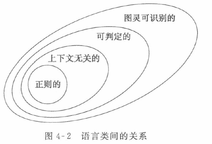
Regular languages sit at the bottom level (Type-3) of the Chomsky Hierarchy, which is the weakest but also the easiest to analyze:

Type-0: Recursively enumerable languages (Turing Machines)
Type-1: Context-sensitive languages (Linear-Bounded Automata)
Type-2: Context-free languages (Pushdown Automata)
Type-3: Regular languages (Finite Automata)

Therefore, after studying regular languages, we proceed to study context-free languages and Turing machines. In terms of containment relationships (the full inclusion hierarchy of language classes) and the corresponding machine capabilities:

Regular languages ⊂ Context-free languages ⊂ Context-sensitive languages ⊂ Turing-decidable languages
Finite automata < Pushdown automata < Linear-bounded automata < Turing machines

1.6 The Pumping Lemma

If we encounter a language L and want to determine what it is, we can follow this line of reasoning:

First, attempt to construct a DFA/NFA/regular expression for the language. If successful, then L is a regular language.
If construction fails, we suspect L might not be regular. We then use the pumping lemma for regular languages to prove the language fails the pumping condition. If successful, the language is not regular.
If the language is not regular, we attempt to construct a pushdown automaton (PDA) or context-free grammar (CFG). If successful, L is a context-free language (CFL).
If construction fails, we suspect the language is not a CFL, so we apply the pumping lemma for context-free languages. If successful, it is not a CFL.
If the language is not context-free, we can continue to determine whether it is a context-sensitive language or a recursively enumerable language; if we can successfully construct a linear-bounded automaton (LBA) or Turing machine, then it belongs to the corresponding class.

At the regular and context-free language levels, the pumping lemma is the most useful tool. However, at the context-sensitive and Turing machine levels, the pumping lemma is no longer as useful. Therefore, we focus here on the pumping lemmas for regular and context-free languages.

The Pumping Lemma for regular languages can be used to prove that a language is not regular. In other words, the pumping lemma is a falsification tool. We can assume a language L is regular, then show that L fails the pumping lemma property to conclude the language is not regular. However, if a language L satisfies the pumping lemma property, we cannot conclude it is regular.

Consider the languages:

\[ B = \{0^n1^n \mid n \geq 0\} \]

\[ C = \{\,w \mid w \text{ 中 }0\text{ 和 }1\text{ 的数量相等}\,\} \]

\[ D = \{\,w \mid w \text{ 中出现子串 }01\text{ 和 }10\text{ 的次数相等}\,\} \]

In the above languages, both 0s and 1s can occur infinitely many times, but it is hard to judge intuitively which are regular and which are not. Among the three: B and C are not regular, but D is regular.

Therefore, we need a practical, rigorous method to determine whether a language is regular.

We typically use the pumping lemma to prove non-regularity. Why is it called the "pumping lemma"? The word "pump" is analogous to inflating a bicycle tire: you push the pump down and pull it back up, repeatedly and rhythmically.

For example, given the string "xyyyyyyz," the middle y can clearly be "pumped" in, so the string can be rewritten as "x{pump:y}z."

Now let us state the Pumping Lemma: If A is a regular language, then there is a number $p > 0$ (the pumping length) where if $s$ is any string in A of length at least $p$, then $s$ may be divided into three pieces, $s = xyz$, satisfying the following conditions:

for each $i \geq 0, xy^{i}z \in A$, where $y^i$ denotes $i$ copies of $y$ concatenated together
$\lvert y \rvert > 0$, where the double bars denote the length of string $y$
$\lvert xy \rvert \leq p$

That $y$ has nonzero length is also written $y \ne \varepsilon$, where $\varepsilon$ specifically denotes the empty string in formal language and automata theory (rendered in LaTeX as \varepsilon). When string $s$ is divided into $xyz$, either $x$ or $z$ may be the empty string, but $y$ cannot be the empty string. This condition is the heart of the pumping lemma. Condition 3 means that the pumpable portion must occur within the first $p$ characters of the string.

In summary, remember these key points:

pumping length p > 0
exist string s, |s| >= p
$xy^{i}z \in A$
|xy|<=p
|y|>0

The proof strategy is:

Obtain p from the pumping lemma
Choose an s with |s| >= p and s in L
List the three properties of the pumping lemma
Decompose s to determine the content of xy
Pump y to obtain s'
Show s' is not in L, completing the proof by contradiction

Now let us revisit the three languages B, C, and D.

EXAMPLE 1

$B = \{0^n1^n \mid n \geq 0\}$

First, assume B is a regular language; then B must satisfy the pumping lemma. Let p > 0 be the pumping length. There must exist a string s with |s| >= p that belongs to B. By the pumping lemma: s = xyz, s' = xy^iz also belongs to B, and |xy| <= p, |y| > 0.

Now, choose n = p, so s = xyz. Since |xy| <= p, xy contains only 0s, and therefore y also contains only 0s. Now, by the pumping lemma, let i = 2, so s' = xyyz also belongs to B. Since y contains only 0s, s' has more 0s than s — at least one additional 0. Since z is unchanged and all 1s are in z, the number of 1s in s' is the same.

We find that xyyz has unequal numbers of 0s and 1s, so xyyz does not belong to B. This contradicts our assumption, so B is not a regular language.

EXAMPLE 2

$C = \{\, w \mid w \text{ has an equal number of }0\text{s and }1\text{s} \,\}$.

This can be proved directly using the counterexample from B, since C is a generalization of B (B is a special case of C), so the same counterexample applies.

EXAMPLE 3

\[ F = \{\, ww \mid w \in \{0,1\}^* \,\} \]

This is quite similar to the above. We can double the construction from B to form a special case, then derive a contradiction.

Let $s=0^p1^p0^p1^p$, so |s| = 4p >= p. Decompose s into xyz. Since |xy| < p, xy contains only 0s. Since |y| > 0, y consists only of 0s. Now pump with i = 2: s' = xyyz. The new string has more 0s, causing the first half $0^{p+\text{extra}}1^p$ and the second half $0^p1^p$ to have unequal lengths. Thus s' does not belong to F, contradicting our assumption, which proves F is not a regular language.

EXAMPLE 4

$D = \{\, 1^{n^{2}} \mid n \geq 0 \,\}$

This language consists solely of strings of 1s whose length is a perfect square $n^2$.

Proof: Let n = p, decompose s into s = xyz, and let i = 2. Then $s'=xyyz, |s'|=|s|+|y|=p^2+k$. Our task is to show that $p^2+k$ is not a perfect square. Since p is an integer, the next perfect square after $p^2$ is $(p+1)^2 = p^2+2p+1$. Since $1 \leq \lvert y \rvert \leq p$, we have $p^2 < p^2 + k \leq p^2+p < p^2 + 2p + 1$. Therefore, after pumping, the length falls strictly between two consecutive perfect squares and hence is not itself a perfect square. This proves D is not a regular language.

EXAMPLE 5

Proving a language is not a palindrome language.

This type of proof can use the closure property: if L is not a palindrome language and is regular, then its complement is also regular. We then only need to show that the complement of L (the palindrome language) is not regular.

Ch.2 Context-Free Grammars

2.1 CFL

At the end of Chapter 1, we learned how to use the pumping lemma to prove a language is not regular. A classic example:

\[ \{0^n1^n \mid n \ge 0\} \]

Since the counts of 0s and 1s are both unlimited and indeterminate, we cannot construct a DFA to describe this language. In this chapter, we study a context-free grammar (CFG) that can describe such languages. In the Chomsky Hierarchy, CFGs occupy Level 2 (Type-2):

Type-0: Recursively enumerable languages (Turing Machines)
Type-1: Context-sensitive languages (Linear-Bounded Automata)
Type-2: Context-free languages (Pushdown Automata)
Type-3: Regular languages (Finite Automata)

Context-free grammars have important applications in programming languages. When language designers build compilers and interpreters, they often need the grammar of the language first. Therefore, most compilers and interpreters contain a parser that extracts the semantics of a program before generating compiled code or interpreting execution.

The class of languages associated with context-free grammars is called context-free languages (CFL). Note that context-free languages include all regular languages.

A context-free grammar consists of a set of substitution rules, also called productions. Each rule occupies one line and consists of a symbol and a string.

For example, grammar $G_1$:

\[ \begin{aligned} A &\rightarrow 0A1 \\ A &\rightarrow B \\ B &\rightarrow \# \end{aligned} \]

The three rules above are substitution rules (or productions). They mean:

An A can become the combination of a 0, an A, and a 1
An A can also become a B
A B can become a #

Symbols that can be replaced are called variables or non-terminals. In the example above, A and B can be replaced, so A and B are variables.

Symbols that cannot be further replaced are called terminals. These irreplaceable symbols are the basic building blocks in the derivation process and form the components of the final product. In the grammar above, the terminals are 0, 1, and #.

The start variable is the starting point for derivation. By convention, it is the variable on the left side of the first rule — in the grammar above, it is A.

How do we use this grammar to derive strings? Starting from the start variable A, we repeatedly apply rules to perform substitutions until we obtain a string containing only terminals. For example:

Start from A; goal is to derive the string 00#11
A
0A1
0(0A1)1
00B11
00#11 — derivation complete

This process is called a derivation. Any string that can be produced through this derivation process conforms to the grammar and is part of the language of the grammar. A language that can be generated by a context-free grammar is called a context-free language (CFL).

The key property of the grammar example above is that the number of 0s and 1s on either side of the # must be equal. Written as a language:

\[ \{0^n\#1^n \mid n \ge 0\} \]

Any string that violates this pattern cannot be produced by this grammar, for example:

00#1
01#
0011
a#b

For convenience, we write variables with multiple production alternatives as:

\[ \begin{aligned} A &\rightarrow 0A1 | B\\ B &\rightarrow \# \end{aligned} \]

2.2 CFG

The formal definition of a context-free grammar is a 4-tuple:

Set of Variables: $V$
Set of Terminals: $\Sigma$
Set of Rules: $R$
Start Variable: $S$

For example:

\[ \begin{aligned} &\text{Set of Variables (V): } V = \{P\} \\ &\text{Set of Terminals } (\Sigma): \Sigma = \{a, b, (, ), \cup, *, \emptyset\} \\ &\text{Set of Rules (R):} \\ &P \rightarrow a \\ &P \rightarrow b \\ &P \rightarrow \emptyset \\ &P \rightarrow (P) \\ &P \rightarrow P \cup P \\ &P \rightarrow PP \\ &P \rightarrow P* \\ &\text{Start Variable (S): } S = P \end{aligned} \]

Example 1: Equal-count language type

$L_1 = \{ a^n b^n \mid n \ge 0 \}$

The number of $a$'s must exactly equal the number of $b$'s, and all $a$'s must precede all $b$'s.

\[ S \to a S b \mid \varepsilon \]

The rule $S \to a S b$ ensures that every $a$ generated is eventually paired with a surrounding $b$. This nesting structure guarantees that the counts of $a$'s and $b$'s grow in lockstep.

Example 2: Palindromes

$L_2 = \{ w \mid w = w^R, w \in \{0, 1\}^* \}$

The string is a palindrome (reads the same forwards and backwards), and may have odd or even length.

\[ S \to 0 S 0 \mid 1 S 1 \mid 0 \mid 1 \mid \varepsilon \]

The rules $S \to 0 S 0$ and $S \to 1 S 1$ ensure that the outermost characters are always identical (recursively shrinking toward the center). $S \to 0$, $S \to 1$, $S \to \varepsilon$ provide the termination points for odd-length and even-length palindromes.

Example 3: Matching and nesting (balanced parentheses)

$L_3 = \{ w \mid w \text{ is a correctly matched string of } ( \text{ and } ) \}$

The string consists of parentheses that must be correctly matched and may be nested or juxtaposed.

\[ \mathbf{CFG:}\quad S \to ( S ) \mid S S \mid \varepsilon \]

Nesting rule $S \to ( S )$: Ensures a matching pair of parentheses can wrap another matched structure.
Concatenation rule $S \to S S$: Ensures two valid matched strings can be juxtaposed (e.g., deriving $(\mathbf{()}) \mathbf{()}$ from $(~)$).
Base rule $S \to \varepsilon$: Provides the empty string as a termination point for derivations.

Example 4: Symmetric ends with arbitrary middle

*$L_5 = { w a w^R \mid w \in {0, 1}^* }$ *

The string begins with an arbitrary substring $w$, ends with the reverse $w^R$, and has a fixed separator $a$**** in the middle.

\[ \mathbf{CFG:}\quad S \to 0 S 0 \mid 1 S 1 \mid a \]

Symmetry rules $S \to 0 S 0$ and $S \to 1 S 1$: Ensure the outer symmetry between $w$ and $w^R$, recursively shrinking toward the center.
Termination rule $S \to a$: When recursion ends, the center must be the fixed separator $a$.
- Note: If the language allows $w$ to be empty ($w = \varepsilon$), then $S \to a$ also serves as the base case.

Proof of Correctness (CFG)

For a CFG, we need to prove:

Every string generated by the CFG is in L
Every string in L can be generated by the CFG

For (1), we can demonstrate by direct derivation.

For (2), we can set up a base case, then use the inductive step to show that the case for $k$ extends to $k+1$.

2.3 Pushdown Automata

A PDA is similar to an FA: it also has ordinary states, an initial state, and accept states. However, in addition to the FA's structure, a PDA's transitions involve:

Input
Pop
Push

These are typically written as: Input, Pop/Push

See the textbook or online resources for details. Note that when proving equivalences, CFG (Context-Free Grammar) and PDA are equivalent; in general, CFGs are somewhat easier to construct.

Ch.3 Turing Machines

3.1 Turing Machines

3.2 Formal Definition

A Turing machine consists of a 7-tuple. Using a binary increment Turing machine as an example:

Set of States (Q):

$$ Q = {Start, Carry, Back, End} $$ 2. Input Alphabet (Σ):

$$ \Sigma = {0, 1} $$ 3. Tape Alphabet (Γ):

$$ \Gamma = {0, 1, -} $$ 4. Transition Function (δ):

$$ \begin{aligned} \delta(Start, 0) &= (Start, 0, R) \ \delta(Start, 1) &= (Start, 1, R) \ \delta(Start, -) &= (Carry, -, L) \[6pt] \delta(Carry, 1) &= (Carry, 0, L) \ \delta(Carry, 0) &= (Back, 1, L) \ \delta(Carry, -) &= (Back, 1, L) \[6pt] \delta(Back, 0) &= (Back, 0, L) \ \delta(Back, 1) &= (Back, 1, L) \ \delta(Back, -) &= (End, -, R) \end{aligned} $$ 5. Start State:

$$ q_0 = Start $$ 6. Accept State:

$$ q_{\text{accept}} = End $$ 7. Reject State:

$$ q_{\text{reject}} = \emptyset $$

3.3 The Church-Turing Thesis

In 1900, the mathematician Hilbert presented 23 mathematical problems at the International Congress of Mathematicians in Paris. The tenth of these concerned the solvability of Diophantine equations — that is, given an indeterminate equation:

\[ a_1 x_1^{b_1} + a_2 x_2^{b_2} + \cdots + a_n x_n^{b_n} = c \]

Hilbert's question was: can we determine, given an arbitrary Diophantine equation with any number of unknowns, whether the equation has integer solutions through a feasible method (what Hilbert called a Verfahren — what we today call an algorithm) in a finite number of steps?

Although people had known about algorithmic procedures like the Euclidean algorithm since ancient Greece and the Spring and Autumn period in China, even by Hilbert's time there was still no precise concept of what constitutes a feasible computation. What it means for a problem to be solvable or unsolvable was not yet understood.

In 1936, Church (Alonzo Church) and Turing (Alan Turing) provided definitions for this question. Church used a notation system called the $\lambda$-calculus to define algorithms, while Turing used machines to do the same thing. These two definitions were later proved to be equivalent, and the connection between the informal notion of algorithms and the precise definition has since been called the Church-Turing Thesis:

Intuitive notion of algorithms

EQUALS

Turing machine algorithms

In short, the Church-Turing Thesis asserts: any problem we intuitively consider computable, or any problem for which an algorithm exists, is equivalent to being solvable by a Turing machine.

The definition of algorithm proposed by the Church-Turing Thesis was essential for resolving Hilbert's 10th problem. In 1970, Matiyasevich proved that the problem is unsolvable.

Ch.4 Decidability

1761016039627

4.1 Recognizable Languages

See the next section for details.

4.2 Decidable Languages

We say that a Turing machine $M$ accepts $w$ when the machine starts from an initial configuration $C_1$ (i.e., the machine is in initial state $q_0$, the tape contains $w$, and the read/write head is at the beginning of $w$) and runs through a sequence of single-step transitions ($C_i$ yields $C_{i+1}$), ultimately reaching an "accept configuration" $C_k$ (i.e., the machine's state becomes $q_{\text{accept}}$). As long as such a path to $q_{\text{accept}}$ exists, we say $M$ accepts $w$.

Based on the definition of "accept," we can define the "language" of a Turing machine:

Definition: The language of a Turing machine $M$, denoted $L(M)$, is the set of all strings $w$ that $M$ accepts.
Mathematical notation: $L(M) = \{w \mid M \text{ accepts } w\}$

Now, based on the concept of $L(M)$, we define two different "levels" of languages:

(A) Turing-recognizable language

Definition: A language $L$ is Turing-recognizable if there exists a Turing machine $M$ such that $L(M) = L$.
Informal explanation:
- If a string $w$ is in the language $L$ (i.e., $w \in L$), then this Turing machine $M$ will halt and accept $w$.
- If a string $w$ is not in the language $L$ (i.e., $w \notin L$), then $M$ has two possible behaviors:
  1. Halt and reject.
  2. Never halt (enter an infinite loop).
Key point: Such a machine only needs to give an affirmative response (halt and accept) for "yes" answers ($w \in L$). It need not guarantee halting for "no" answers.

(B) Turing-decidable language

Definition: A language $L$ is Turing-decidable if there exists a "decider" $M$ that decides it.
What is a "decider"?
- A "decider" is a special type of Turing machine that guarantees it will never enter an infinite loop on any input. It always halts within finite time and gives an "accept" or "reject" answer.
Informal explanation:
- If a string $w$ is in the language $L$ (i.e., $w \in L$), the decider $M$ will halt within finite time and accept.
- If a string $w$ is not in the language $L$ (i.e., $w \notin L$), the decider $M$ will also halt within finite time and reject.
Key point: Such a machine (decider) must halt and give a definite answer within finite time for all inputs (whether "yes" or "no").

Property	Turing-recognizable	Turing-decidable
For $w \in L$ (in the language)	Must halt and accept	Must halt and accept
For $w \notin L$ (not in the language)	May halt and reject, or may loop forever	Must halt and reject
Always halts?	Not necessarily	Yes, always halts

In summary, a decider must always halt — that is, no matter what problem (input) you give it, it must complete its computation within finite time and then indicate:

Accept — representing "yes"
Reject — representing "no"

A decider always halts on all inputs and never falls into an infinite loop or endless computation. If a problem can be answered by a decider, then the problem is decidable.

If a language L and its complement are both recognizable, then L is decidable (because we can run two recognizers in parallel — one for L and one for its complement — and one of them will always halt).

Theorem: A language is decidable if and only if it is both Turing-recognizable and co-Turing-recognizable. In other words, a language is decidable if and only if both it and its complement are Turing-recognizable.

Example 1: "Is this number $N$ even?"

How the decider works:

Receive the number $N$.
Compute the remainder of $N$ divided by 2.
If the remainder is 0, halt and answer "yes".
If the remainder is 1, halt and answer "no".

Analysis: This process is very fast, and for any number $N$, it is guaranteed to halt and give a definite "yes" or "no" answer. Therefore, this is a decider.

Example 2: Let $M$ be a Turing machine and $w$ be a string in $M$'s input alphabet. Consider the following problem:

$A = \{\langle M, w \rangle \mid M \text{ moves its head left at some point during its computation on } w\}$

Prove that $A$ is decidable.

Solution:

To prove a language is decidable, we must construct a decider. This decider is a Turing machine that must halt on any input and give the correct "accept" or "reject" answer.

The core difficulty of this problem is: how do we handle the case where $M$ loops forever on $w$?

We construct a decider $D$ that decides language $A$: $A = \{\langle M, w \rangle \mid M \text{ moves left at least once during its computation on } w\}$

We will construct a decider $D$. $D$ will simulate $M$ on $w$, but it will set a maximum step limit to prevent $M$'s infinite loop from causing $D$ itself to loop.

The key is proving: if $M$ never moves left, it will either halt within a finite number of steps or enter a detectable infinite loop.

The decider $D$, upon receiving input $\langle M, w \rangle$, performs the following:

Extract the parameters of $M$ and $w$:

Let $k$ be the number of states of $M$ ($|Q|$).
Let $g$ be the size of $M$'s tape alphabet ($|\Gamma|$).
Let $n$ be the length of $w$ ($|w|$). (If $w$ is the empty string, $n=1$.)

Compute a "maximum steps" bound:

Bound 1 (looping on input $w$): If $M$'s head stays within $w$'s $n$ cells (positions 1 through $n$) and never moves left (i.e., only moves 'R' or 'S'), then its "configuration" is defined by (current state, head position, contents of $n$ cells).

Possible states: $k$
Possible head positions: $n$
Possible tape contents: $g^n$
Total configurations $B_1 = k \times n \times g^n$.
If $M$ runs for more than $B_1$ steps on $w$ and the head never moves past cell $n$, it must have repeated a configuration, meaning it is in a non-left-moving infinite loop.

Bound 2 (looping on blank tape): Once $M$'s head moves past $w$ onto the blank tape (position $> n$) and never moves left, it will never read $w$ again.

Its behavior then depends only on its (current state) and (current tape symbol).
Possible (state, symbol) combinations: $B_2 = k \times g$.
If $M$ runs for more than $B_2$ steps on blank tape (without moving left or halting), it must have repeated a (state, symbol) combination. Since the tape to its right is always the same (all $\sqcup$ or the symbol sequence it has written), it is in a non-left-moving infinite loop.

Total bound: We set a total simulation step count $B = B_1 + B_2$.

Begin the bounded simulation:

Simulate $M$ on $w$, but for at most $B$ steps.
At each step of the simulation:
- Case (a): If $M$'s transition function indicates it moves left (L), then $D$ halts and accepts (ACCEPT). (Because $\langle M, w \rangle \in A$.)
- Case (b): If $M$ halts (enters $q_{\text{accept}}$ or $q_{\text{reject}}$), then $D$ halts and rejects (REJECT). (Because it halted without ever moving left.)
- Case (c): If the simulation reaches $B$ steps and $M$ has neither moved left nor halted.

4. Draw the conclusion:

If case (a) or (b) occurred during simulation, $D$ has already given its answer.
If the simulation reaches $B$ steps (case c), by our analysis of $B_1$ and $B_2$, this necessarily means $M$ has entered a non-left-moving infinite loop. Therefore, $D$ halts and rejects (REJECT).

Why is $D$ a decider?

$D$ always halts: $D$'s simulation either terminates within $B$ steps due to case (a) or (b), or is forcibly stopped at $B$ steps due to case (c). $B$ is a specific, finite number computed from the input $\langle M, w \rangle$. Therefore, $D$ never loops forever.
$D$ is always correct:
If $\langle M, w \rangle \in A$ ($M$ does move left), this move must occur before $M$ halts or loops. If it occurs within $B$ steps, $D$ accepts via case (a). If $M$ were to move left only after $B$ steps, it would have had to enter a loop within $B$ steps — but this is impossible (since our bound $B$ is designed to detect non-left-moving loops), so the left move must occur within $B$ steps.
If $\langle M, w \rangle \notin A$ ($M$ never moves left), $M$ has only two possibilities:
1. $M$ halts: $D$ rejects within $B$ steps via case (b).
2. $M$ loops forever: $D$ detects this loop at $B$ steps via case (c) and rejects.

Therefore, $D$ is a decider, so $A$ is decidable.

Example 3:

$A_{TM}$ is recognizable but not decidable;

$\overline{A_{TM}}$ is neither recognizable nor decidable.

Quiz 3: You will be asked to prove languages decidable or recognizable.

Topics covered:

Decidable languages, corresponding to deciders
Recognizable languages, corresponding to recognizers (semi-deciders)

Note that all decidable languages are recognizable:

A decidable language: accepts and halts on L, rejects and halts on non-L — always halts
A recognizable language: accepts and halts on L, rejects or loops forever on non-L — halting not guaranteed

4.3 The Diagonalization Method

According to COROLLARY 4.18 on textbook, some languages are not Turing-recognizable.

According to the diagonalization method, $L_{diag}$ and its complement is not recognizable.

Ch.5 Reducibility

Reduction is a core concept in the theory of computation and computational complexity theory, used to compare the difficulty of two problems.

If problem A is reducible to problem B, then solving A cannot be harder than solving B — that is, A is no harder than B — because a solution to B yields a solution to A.

For example, the problem of navigating a new city can be reduced to the problem of obtaining a map, since having a map makes navigation much easier. Similarly, the problem of traveling from Boston to Paris can be reduced to buying a plane ticket between the two cities, which in turn can be reduced to earning the money for the ticket, which can further be reduced to finding a job.

In mathematics, measuring the area of a rectangle can be reduced to measuring its length and width; solving a system of linear equations can be reduced to computing the inverse of a matrix.

In computation theory, if A is reducible to B and B is decidable, then A is decidable. At the same time, if A is undecidable and is reducible to B, then B is also undecidable.

Through reduction, we can prove whether a problem is computationally solvable. This proof method is called reducibility.

5.1 Proving Undecidability

In Chapter 4, we discussed how to determine whether a language is decidable: if a problem can be answered by a decider, then the problem is decidable. In this section, we prove that a problem is undecidable: first prove another problem is undecidable, then reduce the original problem to it.

5.2 Proving the Halting Problem Is Undecidable

The halting problem is:

\[ HALT_{TM} = \{\langle M, w \rangle | M \text{ is a Turing machine and } M \text{ halts on input } w\} \]

Compare with $A_{TM}$ (the acceptance problem):

$A_{TM}$ (acceptance problem): $\{\langle M, w \rangle | M$ accepts $w \}$
- It only cares whether $M$ accepts $w$. If $M$ rejects $w$ or loops on $w$, then $\langle M, w \rangle$ is not in $A_{TM}$.
$HALT_{TM}$ (halting problem): $\{\langle M, w \rangle | M$ halts on $w \}$
- It cares whether $M$ halts (regardless of whether the result is accept or reject).
- Only when $M$ loops on $w$ is $\langle M, w \rangle$ not in $HALT_{TM}$.

Example:

Suppose we have a Turing machine $M$ and input $w$.

Behavior of M on w	In ATM?	In HALTTM?
$M$ accepts $w$	Yes	Yes (accepting is a form of halting)
$M$ rejects $w$	No	Yes (rejecting is a form of halting)
$M$ loops forever on $w$	No	No

So the "halting problem" is this question:

"Does there exist a universal algorithm (decider) to which you can give any program (Turing machine $M$) and any input ($w$), and this algorithm always tells you: 'This program will crash (loop forever) on this input' or 'It will eventually halt (producing an accept or reject result)'?"

Proof:

By contradiction.

Assume $HALT_{TM}$ is decidable. If this assumption holds, there must exist a Turing machine — let us call it decider R — that decides $HALT_{TM}$.

R's goal is to determine whether M halts on w:

If M eventually halts on w, R accepts
If M loops forever on w, R rejects

R always halts and gives either an accept or reject answer.

We know that $A_{TM}$ is undecidable, so we use R to construct a machine S that decides $A_{TM}$.

S's goal is to decide whether belongs to $A_{TM}$:

If M accepts w, then S must accept
If M rejects w, then S must reject
If M loops on w, then S must reject

Given input , S passes to R for judgment. S waits for R's answer; since R is a decider, R is guaranteed to halt and give an answer.

R's answer has two cases:

(1) If M does not accept w — i.e., M loops forever on w, or M halts on w and the simulation result is that M rejects w — then S halts and rejects .

(2) If M accepts w — i.e., M halts on w and the simulation result is that M accepts w — then S halts and accepts .

We can see that regardless of R's answer, S always halts. If the simulation result is M rejecting w, S halts and rejects; if the simulation result is M accepting w, S halts and accepts. Therefore S can decide whether M accepts w, meaning S is a decider for $A_{TM}$ — in other words, $A_{TM}$ is decidable.

However, we know that $A_{TM}$ is undecidable, producing a contradiction. This contradiction means our assumption — that $HALT_{TM}$ is decidable — does not hold. We therefore conclude: $HALT_{TM}$ is undecidable.

5.3 Proving L17 Is Undecidable

Using the same method that proved the halting problem undecidable, we can continue to prove other problems undecidable.

$L_{17} = \{X|X \text{ is a Turing machine that accepts at least 17 distinct input strings}\}$

Proof:

By contradiction.

Assume $L_{17}$ is decidable. If this assumption holds, there must exist a Turing machine — let us call it decider $R$ — that decides $L_{17}$.

$R$'s goal is to determine whether Turing machine $X$ accepts at least 17 strings:

If $X$ accepts $\ge 17$ strings, $R$ accepts $\langle X \rangle$.
If $X$ accepts $< 17$ strings, $R$ rejects $\langle X \rangle$.

$R$ always halts and gives either an accept or reject answer.

We know that $A_{TM}$ is undecidable, so we use $R$ to construct a machine $S$ that decides $A_{TM}$.

$S$'s goal is to decide whether $\langle M, w \rangle$ belongs to $A_{TM}$:

If $M$ accepts $w$, then $S$ must accept.
If $M$ rejects $w$, then $S$ must reject.
If $M$ loops on $w$, then $S$ must reject.

Given input $\langle M, w \rangle$, S constructs a new Turing machine D. D is designed so that when given any input string x, it ignores x and instead simulates M on w:

If M accepts w, then D accepts x.
If M rejects or loops on w, then D rejects x.

After construction, $S$ passes D's result to $R$ for judgment. $S$ waits for $R$'s answer; since $R$ is a decider, $R$ is guaranteed to halt and give an answer.

$R$'s answer has two cases:

(1) If M does not accept w — i.e., M loops forever on w, or M halts but rejects w — then D rejects x, meaning D accepts 0 strings. Therefore R determines 0 < 17, so R rejects D's result, and S halts and rejects .

(2) If M accepts w — i.e., M halts and accepts w — then D accepts x, meaning D accepts all strings (a number far greater than 17). Therefore R determines > 17, so R accepts D's result, and S halts and accepts .

We can see that regardless of $R$'s answer, $S$ always halts.

If $M$ does not accept $w$ (rejects or loops), $S$ halts and rejects.
If $M$ accepts $w$, $S$ halts and accepts.

Therefore $S$ can decide whether $M$ accepts $w$, meaning $S$ is a decider for $A_{TM}$ — in other words, $A_{TM}$ is decidable.

However, we know that $A_{TM}$ is undecidable, producing a contradiction. This contradiction means our assumption — that $L_{17}$ is decidable — does not hold. We therefore conclude: $L_{17}$ is undecidable.

5.4 Proving M17 Is Undecidable and Unrecognizable

$M_{17} = \{X|X \text{ is a Turing machine that accepts at most 17 distinct input strings}\}$

Proof:

By contradiction.

Assume $M_{17}$ is decidable. If this assumption holds, there must exist a Turing machine — let us call it decider $R$ — that decides $M_{17}$.

$R$'s goal is to determine whether Turing machine $X$ accepts at most 17 strings:

If $X$ accepts $\le 17$ strings, $R$ accepts $\langle X \rangle$.
If $X$ accepts $> 17$ strings, $R$ rejects $\langle X \rangle$.

$R$ always halts and gives either an accept or reject answer.

We know that $A_{TM}$ is undecidable, so we use $R$ to construct a machine $S$ that decides $A_{TM}$.

$S$'s goal is to decide whether $\langle M, w \rangle$ belongs to $A_{TM}$:

If $M$ accepts $w$, then $S$ must accept.
If $M$ rejects $w$, then $S$ must reject.
If $M$ loops on $w$, then $S$ must reject.

Given input $\langle M, w \rangle$, $S$ constructs a new Turing machine $D$. $D$ is designed so that when given any input string $x$, it ignores $x$ and simulates M on w:

If $M$ accepts $w$, then $D$ accepts $x$.
If $M$ rejects or loops on $w$, then $D$ rejects $x$.

After construction, $S$ passes $D$'s result to $R$ for judgment. $S$ waits for $R$'s answer; since $R$ is a decider, $R$ is guaranteed to halt and give an answer.

$R$'s answer has two cases:

(1) If $M$ does not accept $w$ — i.e., $M$ loops forever on $w$, or $M$ halts but rejects $w$ — then $D$ rejects $x$, meaning $D$ accepts 0 strings. Therefore $R$ determines $0 \le 17$, so $R$ accepts $\langle D \rangle$, and $S$ halts and rejects $\langle M,w \rangle$.

(2) If $M$ accepts $w$ — i.e., $M$ halts and accepts $w$ — then $D$ accepts $x$, meaning $D$ accepts all strings (a number far greater than 17). Therefore $R$ determines $> 17$, so $R$ rejects $\langle D \rangle$, and $S$ halts and accepts $\langle M, w \rangle$.

We can see that regardless of $R$'s answer, $S$ always halts.

If $M$ does not accept $w$ (rejects or loops), $S$ halts and rejects.
If $M$ accepts $w$, $S$ halts and accepts.

Therefore $S$ can decide whether $M$ accepts $w$, meaning $S$ is a decider for $A_{TM}$ — in other words, $A_{TM}$ is decidable.

However, we know that $A_{TM}$ is undecidable, producing a contradiction. This contradiction means our assumption — that $M_{17}$ is decidable — does not hold. We therefore conclude: $M_{17}$ is undecidable.

Proving M17 is unrecognizable.

Proof:

Assume $M_{17}$ is recognizable.

$\overline{M_{17}} = L_{18} = \{X | X \text{ accepts at least 18 strings}\}$

We must construct a recognizer R18. R18 records accepted input strings x, and once 18 accepted strings have been reached, it immediately halts and accepts x:

If X accepts at least 18 strings, then R18 will halt and accept X.
If X accepts fewer than 18 strings, then R18 will loop forever.

Therefore L18 is recognizable, i.e., the complement of M17 is recognizable. Since we assumed M17 is recognizable, and now its complement is also recognizable, by the theorem, M17 must be decidable.

However, we have already proved that M17 is undecidable, so the assumption leads to a contradiction, meaning M17 is unrecognizable.

5.5 Proving T Is Undecidable

\[ T = \{ \langle M \rangle \mid M \text{ is a Turing machine that accepts } w \text{ if and only if it also accepts } w^R \} \]

where $w^R$ denotes the reverse of string $w$.

Proof:

By contradiction.

Assume $T$ is decidable. If this assumption holds, there must exist a Turing machine — let us call it decider $R$ — that decides $T$.

$R$'s goal is to determine whether Turing machine $X$ satisfies "whenever it accepts $w$, it also accepts $w^R$":

If $X$ satisfies this property (i.e., $w \in L(X) \implies w^R \in L(X)$), $R$ accepts $\langle X \rangle$.
If $X$ does not satisfy this property (i.e., $\exists w$ such that $w \in L(X)$ but $w^R \notin L(X)$), $R$ rejects $\langle X \rangle$.

$R$ always halts and gives either an accept or reject answer.

We know that $A_{TM}$ is undecidable, so we use $R$ to construct a machine $S$ that decides $A_{TM}$.

$S$'s goal is to decide whether $\langle M, w \rangle$ belongs to $A_{TM}$:

If $M$ accepts $w$, then $S$ must accept.
If $M$ rejects $w$, then $S$ must reject.
If $M$ loops on $w$, then $S$ must reject.

Given input $\langle M, w \rangle$, $S$ constructs a new Turing machine $D$. $D$ is designed so that when given any input string $x$, $D$ first simulates $M$ on $w$:

If $M$ accepts $w$, then $D$ checks $x$. If $x = \text{"ab"}$, $D$ accepts $x$; otherwise, $D$ rejects $x$.
If $M$ rejects or loops on $w$, then $D$ rejects $x$ (or loops because $M$ loops).

After construction, $S$ passes $\langle D \rangle$ to $R$ for judgment. $S$ waits for $R$'s answer; since $R$ is a decider, $R$ is guaranteed to halt and give an answer.

$R$'s answer has two cases:

(1) If $M$ does not accept $w$ — i.e., $M$ loops forever on $w$, or $M$ halts but rejects $w$ — then $D$ does not accept any string, i.e., $L(D) = \emptyset$. Therefore $R$ determines that $D$ satisfies $T$'s property (since the condition "whenever $D$ accepts..." is vacuously true), so $R$ accepts $\langle D \rangle$, and $S$ halts and rejects $\langle M,w \rangle$.

(2) If $M$ accepts $w$ — i.e., $M$ halts and accepts $w$ — then $D$ only accepts "ab", i.e., $L(D) = \{\text{"ab"}\}$. $D$ accepts "ab" but does not accept its reverse "ba". Therefore $R$ determines that $D$ does not satisfy $T$'s property, so $R$ rejects $\langle D \rangle$, and $S$ halts and accepts $\langle M, w \rangle$.

We can see that regardless of $R$'s answer, $S$ always halts.

If $M$ does not accept $w$ (rejects or loops), $S$ halts and rejects.
If $M$ accepts $w$, $S$ halts and accepts.

Therefore $S$ can decide whether $M$ accepts $w$, meaning $S$ is a decider for $A_{TM}$ — in other words, $A_{TM}$ is decidable.

However, we know that $A_{TM}$ is undecidable, producing a contradiction. This contradiction means our assumption — that $T$ is decidable — does not hold. We therefore conclude: $T$ is undecidable.

5.6 Proving the "Odd Turing Machine" Language Is Unrecognizable

Call a Turing Machine that accepts input strings in binary odd if it only accepts binary inputs that end in 1. Consider the language

\[ T = \{ \langle M \rangle \mid M \text{ is an odd Turing machine} \} \]

Prove that T is not recognizable.

Proof:

By contradiction.

Assume $T$ is recognizable. If this assumption holds, there must exist a Turing machine — let us call it recognizer $R$ — that recognizes $T$.

$R$'s goal is to determine whether Turing machine $X$ is an "odd" TM:

If $X$ is an "odd" TM (i.e., $X$ only accepts binary strings ending in '1'), $R$ halts and accepts $\langle X \rangle$.
If $X$ is not an "odd" TM (i.e., $X$ accepts at least one string not ending in '1'), $R$ does not accept $\langle X \rangle$ (it may halt and reject, or loop forever).

$R$ is only guaranteed to halt and accept when its input belongs to $T$.

We know that $\overline{A_{TM}}$ is unrecognizable. So we use $R$ to construct a machine $S$ that recognizes $\overline{A_{TM}}$.

($\overline{A_{TM}} = \{\langle M, w \rangle \mid M \text{ does not accept } w\}$)

$S$'s goal is to recognize whether $\langle M, w \rangle$ belongs to $\overline{A_{TM}}$:

If $M$ does not accept $w$ (rejects or loops), then $S$ must accept.
If $M$ accepts $w$, then $S$ must not accept (reject or loop).

Given input $\langle M, w \rangle$, $S$ constructs a new Turing machine $D$. $D$ is designed so that when given any input string $x$:

$D$ first simulates $M$ on $w$.
If $M$ accepts $w$:
- $D$ accepts $x$ (regardless of what $x$ is).
If $M$ rejects or loops on $w$:
- $D$ checks $x$. If $x$ ends in '1', $D$ accepts $x$; otherwise, $D$ rejects $x$ (or loops because $M$ loops).

After construction, $S$ passes $\langle D \rangle$ to $R$ for judgment. $S$ runs $R(\langle D \rangle)$ and mirrors $R$'s behavior (if $R$ accepts, $S$ accepts; if $R$ loops/rejects, $S$ loops/rejects).

$R$'s behavior has two cases:

(1) If $M$ does not accept $w$ (rejects or loops):

In this case, $D$'s simulation never enters the "$M$ accepts $w$" branch. $D$'s behavior is determined by the second branch: it only accepts strings ending in '1'.
(If $M$ loops, $D$ also loops on all inputs $x$, so $L(D) = \emptyset$. The empty language also satisfies "only accepts strings ending in '1'.")
In either case, $D$ is an "odd" TM, i.e., $\langle D \rangle \in T$.
Since $R$ is a recognizer for $T$, $R$ will halt and accept $\langle D \rangle$.
$S$ will halt and accept $\langle M,w \rangle$.

(2) If $M$ accepts $w$:

In this case, $D$'s simulation enters the "$M$ accepts $w$" branch. $D$ will accept all inputs $x$.
$D$'s language $L(D) = \Sigma^*$ (the set of all strings).
$D$ is not an "odd" TM because it accepts strings not ending in '1' (e.g., "0", "10", $\epsilon$). That is, $\langle D \rangle \notin T$.
Since $R$ is a recognizer for $T$, $R$ will not accept $\langle D \rangle$ (it may reject or loop).
$S$ will also not accept $\langle M, w \rangle$.

We can see that $S$'s behavior perfectly matches the definition of $\overline{A_{TM}}$:

If $M$ does not accept $w$, $S$ halts and accepts.
If $M$ accepts $w$, $S$ does not accept.

Therefore $S$ can recognize $\overline{A_{TM}}$, meaning $S$ is a recognizer for $\overline{A_{TM}}$.

However, we know that $\overline{A_{TM}}$ is unrecognizable, producing a contradiction. This contradiction means our assumption — that $T$ is recognizable — does not hold. We therefore conclude: $T$ is unrecognizable.

5.7 Computable Functions

Example Problem

Show that if $A$ is Turing recognizable and $A \le_m \overline{A}$, then $A$ is decidable.

Proof:

Our goal is to prove that $A$ is decidable, which means we need to construct a decider $D_A$. This decider $D_A$ must halt on all inputs $w$ and:

If $w \in A$, then $D_A$ accepts $w$.
If $w \notin A$, then $D_A$ rejects $w$.

By assumption, $A$ is Turing-recognizable. In other words, there exists a Turing machine (recognizer) $R_A$ such that: if $w \in A$, $R_A(w)$ halts and accepts; if $w \notin A$, $R_A(w)$ may halt and reject, or may loop forever.

From the condition $A \le_m \overline{A}$, we know there exists a total computable function $f$ satisfying: $w \in A \iff f(w) \in \overline{A}$.

We can decompose this relationship into two directions:

If $w \in A$, then $f(w) \in \overline{A}$ (i.e., $f(w) \notin A$).
If $w \notin A$, then $f(w) \notin \overline{A}$ (i.e., $f(w) \in A$).

We use $R_A$ and $f$ to construct the decider $D_A$.

Algorithm for $D_A$:

Compute $f(w)$. This step is guaranteed to halt because $f$ is a total computable function.
Run in parallel the following two computations: Run $R_A(w)$ and Run $R_A(f(w))$

When one of the computations halts and accepts:

If $R_A(w)$ accepts, then $D_A$ accepts $w$ and halts.
If $R_A(f(w))$ accepts, then $D_A$ rejects $w$ and halts.

We consider two cases to prove that at least one computation will halt and accept:

Suppose $w \in A$. By assumption, the recognizer $R_A(w)$ will halt and accept. Therefore, $D_A$ will halt.
Suppose $w \notin A$. By assumption, the recognizer $R_A(f(w))$ will halt and accept. Therefore, $D_A$ will halt.

Therefore, $D_A$ always halts.

We again consider both cases and verify that $D_A$'s output is correct:

Suppose $w \in A$. We know $R_A(w)$ will halt and accept, and we know $w \in A \implies f(w) \notin A$. By assumption, $R_A(f(w))$ will never halt and accept (it may reject or loop). Therefore, in the parallel execution, computation 1 must halt and accept first.
Suppose $w \notin A$. We know $f(w) \in A$, so $R_A(f(w))$ will halt and accept. By assumption, since $w \notin A$, $R_A(w)$ will never halt and accept. Therefore, in the parallel execution, computation 2 must halt and accept first.

Thus, we have successfully constructed a Turing machine $D_A$ that always halts on all inputs $w$ and correctly determines whether $w$ belongs to $A$.

Therefore, $D_A$ is a decider for $A$, proving that $A$ is decidable.

Ch.6 The Class P

Starting from this chapter, we enter the topic of complexity theory. Also note that from this chapter onward, the section numbering in my notes will no longer correspond to the textbook's chapter numbering; I will organize sections according to my own needs.

P vs NP, also known as the P/NP problem, is an unsolved problem in the field of computational complexity theory within theoretical computer science. In 2000, the Clay Mathematics Institute (CMI) announced the Millennium Prize Problems with a total prize of $7 million, and the P/NP problem was the first on the list.

Let us review the definitions of P and NP:

P = the class of languages whose membership can be determined quickly
NP = the class of languages whose membership can be verified quickly

The seven Millennium Prize Problems are:

P/NP Problem
Hodge Conjecture
Poincare Conjecture (the only one solved to date)
Riemann Hypothesis
Yang-Mills Existence and Mass Gap
Navier-Stokes Existence and Smoothness
Birch and Swinnerton-Dyer Conjecture

In simple terms, the P/NP problem asks:

Does P equal NP?

This question may appear to have the simplest statement among the seven Millennium Prize Problems, but many believe it will be the last to be solved.

If $P=NP$, then virtually all modern cryptography (RSA, ECC) would instantly fail, a vast number of NP-Hard problems could be solved in linear time or faster, and mathematical automated theorem proving, AI, optimization, and more would undergo revolutionary change. But proving $P \ne NP$ is extremely difficult — it is essentially the ultimate negation of all algorithms, akin to proving "a better method can never be found," which constitutes a proof of inherent difficulty or incomputable structure.

Over the past several decades, researchers have shown that many seemingly powerful mathematical tools known to us cannot resolve the P vs NP problem. In other words, facing P vs NP, we do not even know the direction of entry, let alone which mathematical tool might yield a breakthrough.

6.1 Time Complexity

Why do we need to measure time complexity? Because even if a problem is theoretically decidable, if solving it takes an enormous amount of time — perhaps exceeding the age of the universe since the Big Bang — then even though the problem is decidable, we cannot practically solve it with existing methods. Therefore, we must measure the time required to solve a problem.

Let $M$ be a deterministic Turing machine (i.e., an ordinary computer program that produces a deterministic output for a given input), and let $f(n)$ be M's time complexity function, where:

The input domain is $\mathbb{N}$ (non-negative integers, representing the input string length $n$)
The output domain is $\mathbb{N}$ (non-negative integers, representing the number of steps)

In other words, $f(n)$ is the maximum number of steps that machine $M$ takes when processing any input of length $n$. Here we analyze the worst case.

In addition, we may also analyze the average case.

Big-O

Let $f, g: \mathbb{N} \to \mathbb{R}^+$. We say $f(n) = O(g(n))$ if and only if there exist positive constants $c$ and $n_0$ such that for all $n \ge n_0$:

\[ f(n) \le c \cdot g(n) \]

In other words, as long as $n$ is large enough (exceeds $n_0$) and we allow $g(n)$ to be scaled up by a factor of $c$, $g(n)$ can always "cover" $f(n)$. This means $f$'s growth rate does not exceed $g$'s. In this case, we say $g(n)$ is an asymptotic upper bound of $f(n)$.

The term "asymptotic" here means: we only care about the trend as $n \to \infty$, ignoring the behavior for small $n$ (guaranteed by $n_0$).

Little-o

The difference between little-o and Big-O notation is that in little-o, $f$ grows strictly slower than $g$. In other words, $f(n) = o(g(n))$ means that for any real number $c \gt 0$, there exists a number $n_0$ such that for all $n \ge n_0, f(n) < c g(n)$.

To determine whether $f(n) = o(g(n))$, we typically use the limit test:

\[ \lim_{n \to \infty} \frac{f(n)}{g(n)} = 0 \]

When $n$ tends to infinity, $g(n)$ grows infinitely large relative to $f(n)$, causing their ratio to approach 0. In this case, we say $f(n) = o(g(n))$.

6.2 Polynomial Time

We can memorize the following hierarchy for quick reference when determining time complexity relationships — this is useful in practical programming and problem analysis:

Direction: From top to bottom, growth rate $\uparrow$ (faster toward the bottom).

Constant Time - $O(1)$
- Ex: $1, 100, 5000$ 2. Double Logarithmic - $O(\log \log n)$
- Ex: $\log(\log n)$
- Note: Grows extremely slowly, almost like a constant. 3. Logarithmic - $O(\log n)$
- Ex: $\ln n, \log_2 n$ 4. Polylogarithmic - $O((\log n)^c)$
- Ex: $(\log n)^2, (\log n)^{10}$
- Note: Slower than $O(n)$ but faster than $O(\log n)$. 5. Fractional Power / Sublinear - $O(n^c), 0 < c < 1$
- Ex: $n^{0.5} (\text{i.e., } \sqrt{n}), n^{1/3}$
- Note: Square root always dominates any logarithm. 6. Linear - $O(n)$ 7. Linearithmic / Quasilinear - $O(n \log n)$
- Ex: Merge Sort, Heap Sort 8. Polynomial - $O(n^k), k \ge 1$
- Ex: $n^2$ (Quadratic), $n^3$ (Cubic)
- Note: This is the boundary for "efficient algorithms" (Class P). 9. Quasi-polynomial - $n^{\text{polylog}(n)}$
- Ex: $n^{\log n}$, $2^{(\log n)^c}$
- Characteristics: Base is $n$ but exponent is logarithmic, or base is $2$ but exponent is $\text{polylog}$. 10. Strictly Sub-exponential - $2^{o(n)}$
  - Ex: $h(n) = 2^{\sqrt{n}}$, $2^{n^{1/3}}$
  - Characteristics: Faster than polynomial but not yet as fast as $2^n$. Typically of the form $2^{n^\epsilon}$ ($0 < \epsilon < 1$). 11. Exponential - $O(c^n), c > 1$
  - Ex: $1.01^n, 2^n, e^n, 3^n$
  - Characteristics: Larger base $c$ means faster growth. This is the typical range of "intractable" problems. 12. Factorial - $O(n!)$
  - Ex: Permutation problems
  - Note: By Stirling's approximation, $n! \approx (n/e)^n$, growing extremely fast. 13. Super-exponential - $O(n^n)$
  - Ex: $n^n, 2^{2^n}$ (Double Exponential)
  - Note: The Ackermann function lies in this abyss.

We generally focus on two dividing lines:

Polynomial
Exponential

If a problem has a polynomial algorithm, then given a fast enough computer, we will eventually be able to compute the result. For problems beyond polynomial (super-polynomial), we generally consider them practically intractable.

The exponential level is often used to assess whether a cryptographic algorithm is secure. We generally consider that a cipher breakable in sub-exponential time is practically insecure.

In other words:

Super-polynomial: practically intractable
Sub-exponential: practically insecure

Example Problem

Let us sort the following functions:

Extremely slow growth (logarithmic):
- $f(n) = \log \log n$ (grows extremely slowly, even slower than $\log n$)
Polynomial and below (Polynomials & Roots):
- $d(n) = 2\sqrt{n} + 400,000 \approx O(n^{0.5})$
- $g(n) = 2n^{2/3}\log^2 n \approx O(n^{0.66...})$ (Note: exponent $0.66$ of $n^{2/3}$ is greater than $n^{0.5}$)
- $b(n) = 7n \log n \approx O(n^{1+\epsilon})$ (larger than pure linear, smaller than quadratic)
- $a(n) = 3n^2 + 7 \approx O(n^2)$
- $e(n) = 10n^2 - 40 \approx O(n^2)$
- (Note: $a$ and $e$ are of the same order; they can be placed in either order since $O(a) = O(e)$)
Quasi-polynomial / Sub-exponential:
- Two tricky functions: $l(n) = n^{\log n}$ and $h(n) = 2^{\sqrt{n}}$.
- Transform $l(n)$: $n^{\log n} = 2^{(\log n)^2}$.
- Compare $l(n)$ and $h(n)$: compare the exponent parts $(\log n)^2$ and $\sqrt{n}$. For large $n$, $\sqrt{n}$ far exceeds $(\log n)^2$.
- Therefore: $n^2 < l(n) < h(n)$.
Exponential:
- $j(n) = e^n * n^{23} \approx O(e^n)$ (base $e \approx 2.718$)
- $c(n) = 3^n$ (base $3$)
- Since $e < 3$, we have $j(n) < c(n)$.
Factorial and Doubly Exponential:
- $i(n) = n!$ (by Stirling's approximation, roughly $n^n$, much faster than $3^n$)
- $k(n) = 2^{2^n}$ (doubly exponential, terrifyingly fast growth, placed last)

Final ordering:

\[ f \le d \le g \le b \le a = e \le l \le h \le j \le c \le i \le k \]

.

6.3 The Class P

The class P (Polynomial Time) refers to algorithms that can be completed within polynomial time or less, for example:

$O(1)$
$O(\log n)$
$O(\sqrt{n})$
$O(n)$
$O(n^2)$
$O(n^{100})$

In computer science, the class P is generally considered to represent efficient algorithms.

A convenient way to remember: if the best known algorithm for a problem has worst-case time complexity

\[ O(n^k) \]

where $k$ is some constant and $n$ is the input size, then the problem belongs to the class P.

6.4 Polynomial Equivalence

There are many computational models in the theory of computation (single-tape Turing machines, multi-tape Turing machines, random access machines, etc.). Although their architectures differ, they are typically "polynomially equivalent" — that is, what one model can do, another can also do, with only polynomial overhead for the simulation. Therefore, the class P is robust.

In other words, the scope of $P$ does not depend on the specific computational model (as long as it is deterministic). This demonstrates that $P$ is an objectively existing, mathematically well-defined class rather than an artifact of a particular machine.

$P$ is the class of languages decidable by a deterministic single-tape Turing machine in polynomial time:

\[ P = \bigcup_{k} \text{TIME}(n^k) \]

This encompasses all problems solvable in time complexity $n^1, n^2, n^3 \dots$ and so on.

This discussion of P highlights two important properties:

$P$ is mathematically invariant — a stable set undisturbed by specific implementation details.
$P$ roughly corresponds to the set of practically solvable problems on a computer.

A common question is: "If an algorithm is $n^{100}$, it belongs to P but is practically impossible to run — can we still call it practically solvable?"

The textbook's explanation is:

In practice, very few problems in $P$ can only be solved by algorithms as extreme as $n^{100}$. Typically, once a problem is shown to be in $P$, an $n^2$ or $n^3$ algorithm usually exists.
If a polynomial algorithm is found for a problem that previously seemed to require exponential time (even if it is $n^{100}$), this signals that we have gained insight into the mathematical structure of the problem. The leap from exponential to polynomial is a qualitative change.

In other words, the P vs NP discussion is qualitative in nature. Even if an algorithm runs in $n^{100}$ time, as long as it belongs to P, scientists can typically optimize the algorithm quickly, reducing its exponent (e.g., from $n^{100}$ to $n^3$), ultimately making it practical. Therefore, using polynomial time as the standard for tractability has historically proven to be a very useful rule of thumb.

6.5 Proving Membership in P

Proving that a problem belongs to P amounts to finding a deterministic algorithm whose running time is a polynomial function of the input size. If such an algorithm exists, the decision problem belongs to the complexity class $\mathbf{P}$.

The PATH Problem

The PATH problem discussed in the textbook is essentially graph connectivity. Given a directed graph $G$ containing a set of nodes and a set of edges, along with two specific nodes — a source $s$ and a target $t$ — we need to determine whether there exists a directed path from $s$ to $t$.

Formally, the language is defined as:

\[ PATH = \{ \langle G, s, t \rangle \mid G \text{ is a directed graph containing a directed path from } s \text{ to } t \} \]

The size of the graph is typically measured by the number of nodes $m$.

The brute-force algorithm for this problem searches through all possible paths in $G$ to find one connecting $s$ and $t$. Since a simple path's length cannot exceed the total number of nodes $m$, the brute-force approach attempts to enumerate all node sequences of length at most $m$. However, in a graph with $m$ nodes, the number of possible path combinations is roughly $m^m$. This is exponential growth, meaning that even a slight increase in graph size causes the computation time to explode. Therefore, this brute-force algorithm cannot complete in polynomial time and is not an efficient solution.

To prove that $PATH$ belongs to P, we employ a marking algorithm based on the breadth-first search (BFS) idea. The algorithm's core is to iteratively mark all nodes reachable from the source $s$. The algorithm first marks $s$, then enters a loop: scan all edges in the graph; if an edge leads from a "marked" node to an "unmarked" node, mark the latter as well. This process repeats until no new nodes can be marked.

Since the graph has only $m$ nodes and each effective iteration marks at least one new node, the loop executes at most $m$ times. Each step completes in polynomial time, and the total running time is polynomial in the graph size $m$.

The polynomial-time algorithm is as follows:

Algorithm M (Input: directed graph G, source s, target t)

    1. Initialize: mark node s as "visited."

    2. Loop: repeat the following until no new nodes are marked in a pass:
         For each edge (a, b) in G:
             If node a is marked AND node b is not marked:
                 Mark node b as "visited."

    3. Decision:
         If node t is marked:
             ACCEPT
         Otherwise:
             REJECT

Therefore $PATH \in P$.

The RELPRIME Problem

Another problem mentioned in the textbook is the RELPRIME (relative primality) problem, which determines whether two natural numbers $x$ and $y$ are coprime (i.e., their greatest common divisor is 1):

\[ RELPRIME = \{<x,y>|x \text{ and } y \text{ are relatively prime}\} \]

Formally, if $\gcd(x, y) = 1$, the algorithm accepts the input, where gcd stands for greatest common divisor.

Note that the input size for this problem is defined as the length of the number's representation, not the numerical value itself. For example, if the input size is n, then the input is an n-bit binary number whose numerical range is:

\[ 2^{n-1} \le x < 2^n \]

This range means: the most significant bit must be 1, so the lower bound is $2^{n-1}$, representing an $n$-bit number whose binary representation is $1$ followed by $(n-1)$ zeros ($10\dots0_2$). This is the smallest number requiring exactly $n$ bits. For example, when $n=4$, $2^{4-1} = 2^3 = 8$ (binary $1000_2$). The upper bound $2^n$ is an $(n+1)$-bit number whose binary representation is $1$ followed by $n$ zeros ($10\dots0_2$). All $n$-bit numbers are less than it. For example, when $n=4$, $2^4 = 16$ (binary $10000_2$).

The brute-force approach searches for all common factors of the two numbers. Iterating through all integers from 2 to $\min(x, y)$ to check divisibility is computationally infeasible. For an $n$-bit binary number, its numerical value is approximately $2^n$. If the algorithm's running time is proportional to the numerical value, then relative to the input length $n$, the running time is exponential $O(2^n)$. This kind of linear search based on numerical value is called "pseudo-polynomial time" and is essentially an exponential-time algorithm.

To prove $RELPRIME$ belongs to P, we use the classic Euclidean algorithm (also known as the division algorithm): recursively computing the greatest common divisor using the $x \pmod y$ property. Analysis shows that in the Euclidean algorithm, every two recursive iterations (or two swap operations) reduce the parameter value by at least half. This means the number of iterations is proportional to $\log(\text{value})$. Since $\log(\text{value})$ corresponds exactly to the binary input length, the algorithm's running time is linear or polynomial in the input length, proving the problem is solvable in polynomial time.

The polynomial-time algorithm is as follows:

Algorithm R (Input: natural numbers x, y)

    1. Call subroutine E(x, y) to compute the GCD as follows:
         Algorithm E:
         Repeat until y = 0:
             Let x = x mod y
             Swap x and y
         Output x

    2. Evaluate the output of subroutine E:
         If E's output is 1:
             ACCEPT
         Otherwise:
             REJECT

Therefore $RELPRIME \in P$.

The 2COLOR Problem

Input: an undirected graph $G=(V,E)$ (adjacency list or adjacency matrix)

Output:

If the graph can be 2-colored, output each vertex's color (e.g., RED / BLUE)
If it cannot be 2-colored, report "not bipartite / cannot be 2-colored"

Algorithm:

(1) Initially, every vertex is "uncolored."

(2) For each connected component of the graph, perform one BFS:

Pick any uncolored vertex in the component and color it RED;

Start BFS from it:

For each neighbor v of the current vertex u:

If v is uncolored, assign v the opposite color of u and enqueue it;
If v is already colored and has the same color as u => conflict => cannot 2-color, algorithm terminates with failure.

(3) If all vertices have been checked with no conflicts, return success with the color array.

Ch.7 The Class NP

In the discussion of P-class problems, we saw that many problems can avoid brute-force solutions and achieve polynomial-time solutions. Note that as long as a problem has a polynomial-time solution, it is a P-class problem, regardless of which method you ultimately use to solve it.

However, many problems still have no known polynomial-time solution. In other words, no algorithm that avoids brute force has been found for many problems. Mathematics has not yet been able to explain whether these problems possess an inherent computational hardness.

7.1 NP-Class Problems

Many problems can be solved in polynomial time (P-class problems), but there are also many important problems for which, despite decades of effort, no polynomial-time algorithm has been found. These problems are not understudied — it is possible that no polynomial-time algorithm exists, or that we simply do not yet know how to find one.

Many hard problems are related in complexity:

A polynomial algorithm for one hard problem may be usable to solve another hard problem.

This point is very important for understanding NP-Completeness, but in this section we first discuss the class NP.

Simply put, if P-class problems explore problems solvable in polynomial time, then:

NP-class problems are problems verifiable in polynomial time.

That is, P-class problems are easy to solve, while NP-class problems may not be easy to solve but are easy to check.

The core characteristic of NP problems is polynomial verifiability. We further explore this through the HAMPATH problem below. NP does not stand for "non-polynomial" but rather Nondeterministic Polynomial time:

NP is the class of problems for which a solution can be verified as correct in polynomial time.

7.2 The HAMPATH Problem

HAMPATH (Hamiltonian Path) is a classic problem in graph theory. Given a directed graph $G$ and two specific nodes $s$ (source) and $t$ (target) in the graph, determine whether there exists a path from $s$ to $t$ that visits every node in $G$ exactly once:

\[ \text{HAMPATH} = \{ \langle G, s, t \rangle \mid G \text{ contains a Hamiltonian path from } s \text{ to } t \} \]

In simple terms: Like a traveling salesman who must depart from city $s$, arrive at city $t$, and visit every other city exactly once along the way.

HAMPATH is important because it is a classic NP-complete problem. We will discuss NP-completeness shortly, but regarding the problem itself, it is one of the cornerstones for proving many other complex problems are NP-complete. To date, no one knows of a polynomial-time algorithm to find a Hamiltonian path. The best known algorithms for HAMPATH require exponential time (e.g., $O(2^n)$ or $O(n!)$), making them infeasible for large-scale graphs.

Although HAMPATH is hard to solve in polynomial time, its solutions can be verified in polynomial time:

If someone (the "prover") provides a sequence $P$ claimed to be a Hamiltonian path, we (the "verifier") can check in very short time (polynomial time) whether $P$ is indeed a valid Hamiltonian path:

Check endpoints: Does path $P$ start at $s$ and end at $t$? $\rightarrow O(1)$
Check edge existence: Do the edges between consecutive nodes in $P$ actually exist in graph $G$? $\rightarrow O(n)$ (where $n$ is the number of nodes)
Check node uniqueness: Does path $P$ contain all nodes in $G$ exactly once? $\rightarrow O(n)$

Total complexity: $O(1) + O(n) + O(n) = O(n)$.

Since $O(n)$ is polynomial time, the HAMPATH problem belongs to NP.

7.3 The COMPOSITES Problem

The COMPOSITES problem is a classic example of polynomial verifiability:

\[ \text{COMPOSITES} = \{ x \mid x = pq, \text{ integers } p, q > 1 \} \]

Finding a factor $p$ and $q$ of a large integer is a famously hard problem (no known polynomial-time algorithm exists). But if someone claims $x$ is composite, they only need to provide a factor $p$ of $x$ (satisfying $1 < p < x$).

The verifier only needs to complete two simple checks in polynomial time:

Check that $p$ is greater than 1.
Check that $p$ divides $x$ (i.e., $x \bmod p = 0$).

The verification process is extremely fast, so the COMPOSITES problem is polynomially verifiable and belongs to NP.

7.4 Proving Membership in NP

Verifier

To rigorously define "polynomial verifiability," the textbook introduces the concept of a verifier.

A verifier for language $A$ is an algorithm $V$ where:

\[ A=\{w \mid \text{for some string } c, V \text{ accepts } \langle w, c \rangle \} \]

Since the verifier's time is measured only in terms of the length of $w$, a polynomial time verifier runs in time polynomial in the length of $w$. If a language $A$ has a polynomial time verifier, it is called polynomially verifiable.

The verifier uses additional information (denoted by symbol $c$ in Definition 7.15) to verify that string $w$ is a member of $A$. This information is called a certificate (or proof) of $A$'s membership. Note that for a polynomial time verifier, the certificate has polynomial length (in the length of $w$), since this is all the information the verifier can access within its time bound. Applying this definition to the languages HAMPATH and COMPOSITES:

For the HAMPATH problem, the certificate for the string $\langle G, s, t \rangle \in \text{HAMPATH}$ is simply a Hamiltonian path from $s$ to $t$.
For the COMPOSITES problem, the certificate for a composite number $x$ is simply one of its factors.

In both cases, once the certificate is provided to the verifier, it can check in polynomial time whether the input is in the language.

In summary, to verify that a problem belongs to NP using a verifier, the general steps are:

Define a certificate C, which can be a solution, a subset, etc. C is the evidence proving the problem's answer is "yes."
Set up a Verifier that, through a series of verification steps, decides whether to accept or reject C.
If all verification steps run in polynomial time, then the problem is in NP.

NTM

We can also use a Verifier to prove a problem is in NP.

Theorem:

A language is in NP if and only if it is decided by some nondeterministic polynomial-time Turing machine (NTM).

Being decided by an NTM and being proved via a Verifier are mathematically equivalent.

Proving a language belongs to NP can be done using either a Verifier or an NTM, but the Verifier approach is generally simpler. Let us look at several examples of proving problems belong to NP using verifiers.

The SUBSET-SUM Problem

Proving SUBSET-SUM is in NP

SUBSET-SUM: Given a finite set $S = \{x_1, x_2, \ldots, x_n\}$ where each $x_i$ is a positive integer, and a target positive integer $t$. The SUBSET-SUM language $L$ is the set of all pairs $(S, t)$ satisfying:

\[ L = \{(S, t) \mid \text{there exists a subset } S' \subseteq S \text{ such that the sum of elements in } S' \text{ equals } t \} \]

Proof:

(1) Define the certificate

If an instance (S, t) of language L belongs to the language, there must exist a certificate C.

For this problem, the most natural certificate C is the subset S' whose elements sum to t.

If the answer to SUBSET-SUM is "yes," we can always find this certificate.

Let K be the size of C and N be the size of S.

(2) Verifier verification

We need a verifier to verify that the certificate is valid.

First, the numbers in the certificate must all come from the original set. We can check each number in the certificate to ensure it is in S.

Next, we compute the sum of the certificate's elements and compare it with the target t. If they are equal, the certificate is genuine.

(3) Determine that verification runs in polynomial time

The verification process proceeds as follows:

Look up each number in C within S. For a set S of size N, looking up one number takes O(N) in the worst case, so looking up all of C takes at most O(KN) — polynomial time.
Summing the numbers in C takes O(K) time — polynomial time.
Comparing the sum with t requires a single comparison — polynomial time. If the sum equals t, the verifier accepts C; otherwise it rejects C.

All verification steps can be completed in polynomial time. Therefore, for the original problem, we can always find a certificate C and verify it in polynomial time. By the definition of NP, language L has a polynomial time verifier, so L belongs to NP.

(English version)

Prove:

If some subsets of S sums to exactly t, then we can always find a certificate C, and this certificate is a subset of S and the sum of certificate's elements is t. We can define the subset S' as this certificate.

We need build a verifier to verify this certificate.

First, the numbers in the certificate should come from S. We can check the number in C to judge if they are from S.

Then, we can add the numbers in S', to compare with t. If the sum is the same as t, then SUBSET-SUM is true.

We can define a verifier V, to determine whether we can accept or reject C.

The verification steps are:

(1) Check the number in C to judge if they are from S. There are K numbers in S' and N numbers in S. Then check each number cost N in worst case, so total time we cost is O(KN)

(2) Add the numbers in C, cost O(K)

(3) Compare the sum of C and t, this cost O(1). If the sum is t, then verifier V accept C, otherwise V reject C.

We can see that all verification steps are polynomial time. Therefore, we can verify in polynomial time. So for SUBSET-SUM problem, we can always find a certificate C, and verify in polynomial time. According to definition of NP, SUBSET-SUM now has a verifier can verify in polynomial time, so SUBSET-SUM is in NP.

The 2COLOR Problem

Proving 2COLOR is in NP

2COLOR asks whether a graph can be colored with two colors such that all adjacent vertices have different colors.

\[ \text{2COLOR} = \{G \mid G \text{ has a proper 2-vertex coloring}\} \]

Prove:

For an input graph G, if G has a proper 2-vertex coloring, then there exists a certificate C implementing such a coloring.

We need build a verifier V to verify this certificate C. The verifier V receives the graph G and the certificate C as input.

The verification steps are:

(1) Check all colors in the graph is one of the two valid colors. This cost O(V) time.

(2) Check all vertexes if they have a neighbor has same color. If there exist a situation that two neighbor vertexes have same color, the verifier V immediately reject C. This cost O(V+E) time if we use BFS to traverse the graph, or O(E) time if we can traverse the set of edges.

(3) If there is no rejection happens, after verification, the verifier V accept C.

We can see that all verification steps are polynomial time. Therefore for 2COLOR problem, if the input graph G has a proper 2-coloring, the certificate C can be verified in polynomial time. Hence, by the definition of NP, 2COLOR is in NP.

The 3COLOR Problem

Proving 3COLOR is in NP

3COLOR asks whether a graph can be colored with three colors such that all adjacent vertices have different colors.

\[ \text{3COLOR} = \{G \mid G \text{ has a proper 3-vertex coloring}\} \]

Prove:

For an input graph G, if G has a proper 3-vertex coloring, then there exists a certificate C implementing such a coloring.

We need build a verifier V to verify this certificate C. The verifier V receives the graph G and the certificate C as input.

The verification steps are:

(1) Check all colors in the graph is one of the three valid colors. This cost O(V) time.

(2) Check all vertexes if they have a neighbor has same color. If there exist a situation that two neighbor vertexes have same color, the verifier V immediately reject C. This cost O(V+E) time if we use BFS to traverse the graph, or O(E) time if we can traverse the set of edges.

(3) If there is no rejection happens, after verification, the verifier V accept C.

We can see that all verification steps are polynomial time. Therefore for 3COLOR problem, if the input graph G has a proper 3-coloring, the certificate C can be verified in polynomial time. Hence, by the definition of NP, 3COLOR is in NP.

7.5 coNP

"co" stands for Complement. coNP is the set of all languages whose complement belongs to NP. The definition of $coNP$:

\[ coNP = \{ L \mid \overline{L} \in NP \} \]

A language $L$ belongs to $coNP$ if and only if its complement $\overline{L}$ belongs to $NP$.

Prove: if $P = NP$ then $NP = coNP$

Proof of the above:

By the set-theoretic definition, to prove $A = B$, we need to prove $A \subseteq B$ and $B \subseteq A$. We will use the assumption $P = NP$ along with a key property of the deterministic polynomial time class ($P$): if you can solve a problem deterministically in polynomial time, you can certainly solve its negation (i.e., its complement) in polynomial time.

Assumption: $P = NP$.

Part 1: Prove $NP \subseteq coNP$****

Take any language $L \in NP$.
By the assumption $P = NP$, since $L \in NP$, we have $L \in P$.
By the lemma ($P$ is closed under complement — this key property is easy to prove: for a deterministic Turing machine, simply swap "accept" and "reject" to show P is closed under complement), since $L \in P$, we have $\overline{L} \in P$.
Using the assumption $P = NP$ again, since $\overline{L} \in P$, we have $\overline{L} \in NP$.
By the definition of $coNP$, since $L$'s complement $\overline{L} \in NP$, we have $L \in coNP$.
In summary, for any $L \in NP$ we have $L \in coNP$, therefore $NP \subseteq coNP$.

Part 2: Prove $coNP \subseteq NP$****

Take any language $L \in coNP$.
By the definition of $coNP$, this means $\overline{L} \in NP$.
By the assumption $P = NP$, since $\overline{L} \in NP$, we have $\overline{L} \in P$.
By the lemma ($P$ is closed under complement), since $\overline{L} \in P$, its complement $\overline{\overline{L}}$ (i.e., $L$) also belongs to $P$, meaning $L \in P$.
Using the assumption $P = NP$ again, since $L \in P$, we have $L \in NP$.
In summary, for any $L \in coNP$ we have $L \in NP$, therefore $coNP \subseteq NP$.

Conclusion:

Since we proved $NP \subseteq coNP$ and $coNP \subseteq NP$, we conclude:

If $P = NP$, then $NP = coNP$.

Ch.8 NP-Completeness

NP-Complete is a subset of NP, comprising the hardest problems within NP.

1763842819509

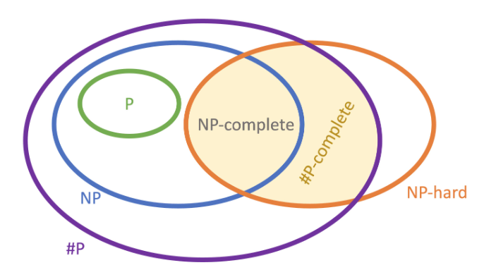
8.1 The Satisfiability Problem

In the 1970s, Stephen Cook and Leonid Levin discovered that the complexity of certain problems in NP is linked to the complexity of the entire class NP: if any NP-complete problem has a polynomial-time algorithm, then all NP problems have polynomial-time algorithms (i.e., $P=NP$).

In other words, on the theoretical side, researchers studying $P \ne NP$ can focus their efforts on finding a non-polynomial-time proof for a single NP-complete problem. On the practical side, NP-completeness prevents people from wasting time searching for polynomial-time algorithms that do not exist.

The first problem proved to be NP-complete was the satisfiability problem (SAT):

\[ SAT = \{\langle \phi \rangle \mid \phi \text{ is a satisfiable Boolean formula}\} \]

Theorem: $SAT \in P$ if and only if $P=NP$.

This theorem states that if the SAT problem can be solved in polynomial time, then all NP problems can be solved in polynomial time, meaning $P$ equals $NP$. And vice versa.

8.2 Polynomial-Time Reducibility

A function $f: \Sigma^* \to \Sigma^*$ is called a polynomial-time computable function if there exists a polynomial-time Turing machine $M$ such that on any input $w \in \Sigma^*$, $M$ halts with exactly $f(w)$ on its tape. The function $f$ can be computed in polynomial time. This is the foundation of "efficient" transformation.

Language $A$ is said to be polynomial-time mapping reducible to language $B$ (polynomial-time reducible for short), written $A \le_p B$, if there exists a polynomial-time computable function $f: \Sigma^* \to \Sigma^*$ such that for every $w$:

\[ w \in A \iff f(w) \in B \]

The function $f$ is called a polynomial-time reduction from $A$ to $B$. $f$ is a mapping from the input domain of set $A$ to the input domain of set $B$. To determine whether a string $w$ belongs to $A$, one only needs to compute $f(w)$ in polynomial time and then determine whether $f(w)$ belongs to $B$.

$A \le_p B$ means: problem $A$ is no harder to solve than problem $B$ (in the sense of polynomial-time complexity). If $B$ has an efficient (polynomial-time) solution, then $A$ can also be solved efficiently through reduction to $B$.

Theorem: If $A \le_p B$ and $B \in \mathbf{P}$, then $A \in \mathbf{P}$.

$\mathbf{P}$ is the set of polynomial-time solvable languages.

Proof sketch:

Let $M$ be the polynomial-time algorithm (Turing machine) that decides $B$.
Let $f$ be the polynomial-time reduction function from $A$ to $B$.
Construct an algorithm $N$ that decides $A$ as follows:
- Input $w$.
- Compute $f(w)$* (completed in polynomial time since *$f$ is a polynomial-time computable function).
- Run $M$ on input $f(w)$* (completed in polynomial time since *$M$ is a polynomial-time algorithm).
- Output $M$'s result.
The total running time of algorithm $N$ is the composition of the polynomial time for computing $f(w)$ and the polynomial time for running $M$, which is still polynomial time.
Therefore $A$ is polynomial-time solvable, i.e., $A \in \mathbf{P}$.

To introduce important reduction examples that follow, the textbook introduces several concepts about Boolean formulas:

Literal: A Boolean variable (e.g., $x$) or its negation (e.g., $\bar{x}$).
Clause: Several literals connected by $\lor$ (or).
Conjunctive normal form (cnf): Several clauses connected by $\land$ (and).
3cnf formula: A formula in which every clause has exactly three literals.
- Example: $(x_1 \lor \bar{x}_2 \lor x_3) \land (\bar{x}_1 \lor x_4 \lor \bar{x}_5)$
3SAT problem: Given a 3cnf formula $\phi$, does there exist a Boolean assignment that satisfies $\phi$ (i.e., makes $\phi$ evaluate to True)? The textbook later provides a proof that 3SAT is polynomial-time reducible to CLIQUE.

8.3 NP-hard

If a problem is classified as NP-Hard, it means it is at least as hard as all the "hard to solve but easy to verify" problems (NP-class problems) in the world.

Note that NP-Hard is not a subset of NP. Some NP-Hard problems are in NP, while others are even harder than NP (even verifying answers cannot be done in polynomial time).

If every NP problem (NxN Sudoku, Hamiltonian path, Tetris, ...) can be "transformed" (reduced) to problem X, then problem X is NP-Hard. If an NP-Hard problem can be solved quickly (in polynomial time), then all NP problems can be solved quickly (in polynomial time).

In other words, if any NP-Hard problem can be solved in polynomial time, then we have proved P = NP.

8.4 NP-Completeness

A language $B$ is called NP-complete if it satisfies the following two conditions:

$B$ belongs to NP:
- This means for any given input, if it is a "yes" instance of $B$, there exists a certificate (or "solution") that can be verified in polynomial time to confirm the input indeed belongs to $B$.
Every language $A$ in NP is polynomial-time reducible to $B$ ($\text{A} \le_p \text{B}$):
- This means $B$ is one of the "hardest" problems in NP. If we can efficiently (in polynomial time) solve $B$, then we can efficiently solve every other problem in NP.
- Polynomial-time reducibility ($\le_p$): There exists a polynomial-time computable function $f$ such that for all inputs $w$, $\text{w} \in \text{A} \iff f(w) \in \text{B}$.

Theorem: P = NP and NP-Completeness:

If the above $B$ is NP-complete and $B \in \mathbf{P}$, then $\mathbf{P} = \mathbf{NP}$.

The class P (Polynomial time): the set of problems solvable in polynomial time.
An NP-complete language $B$ is the hardest problem in NP.
If the hardest $B$ can actually be solved in polynomial time (i.e., $B \in \mathbf{P}$), then by Definition 7.27's condition 2 (all NP languages can be reduced to $B$), all problems in NP can be solved in polynomial time.
Therefore, this proves that P and NP are the same set, i.e., $\mathbf{P} = \mathbf{NP}$.

Theorem: Transitivity of NP-Completeness:

If the above $B$ is NP-complete, $B \le_p C$, and $C$ belongs to NP, then $C$ is NP-complete.

Proof sketch: To prove $C$ is NP-complete, we need to establish two conditions:

$C$ belongs to NP: This is given.
Every language in NP is reducible to $C$****:

Since $B$ is NP-complete, any language $A$ in NP can be polynomial-time reduced to $B$ ($A \le_p B$).
Since $B$ can be polynomial-time reduced to $C$ ($B \le_p C$).
Polynomial-time reducibility is composable (or transitive): if $A \le_p B$ and $B \le_p C$, then $A \le_p C$.
Therefore, every language $A$ in NP can be polynomial-time reduced to $C$.

This shows that as long as a language $C$ is an NP language and is at least as hard as (or harder than) a known NP-complete problem, then $C$ is also NP-complete. This is the primary method for proving new problems are NP-complete.

Brief summary:

NP-complete problems are the hardest problems in NP.
If any NP-complete problem is proved to be solvable in polynomial time, then all NP problems can be solved in polynomial time ($\mathbf{P} = \mathbf{NP}$).
To prove a new problem $C$ is NP-complete, one typically shows that some known NP-complete problem can be polynomial-time reduced to $C$ (while $C$ belongs to NP).

8.5 The Cook-Levin Theorem

The Cook-Levin theorem is a cornerstone of computational complexity theory. It answers the question of whether the concept of "NP-completeness" actually exists and lays the foundation for discovering other NP-complete problems.

8.6 Known NP-Complete Problems

3-SAT

3-Coloring

Vertex Cover

Theorem: VERTEX-COVER is NP-complete.

HAMPATH

Theorem 1: HAMPATH is NP-complete.

Theorem 2: UHAMPATH is NP-complete.

CLIQUE

Subset Sum

Theorem: SUBSET-SUM is NP-complete.

8.7 Proving NP-Completeness

NP-Complete is the intersection of NP and NP-Hard. Therefore, to prove a problem is NP-Complete, one must simultaneously prove:

The problem belongs to NP
The problem belongs to NP-Hard

Proving membership in NP can refer to the section on proving NP membership in these notes; it is typically done using a polynomial-time verifiable certificate.

Proving NP-Hardness is more difficult. A problem being NP-Hard means it is at least as hard as all currently known NP problems. We cannot directly prove this for all NP problems. Instead, we use polynomial-time reduction to reduce a known NP-Complete problem A to the problem L we want to prove. The core logic is to show $A \le_p L$ (known problem $\le$ your problem) — i.e., if you can efficiently solve $L$, you can leverage that solution to efficiently solve $A$. Since $A$ is already hard, $L$ must be equally hard (or harder).

Note that we must reduce a known hard problem to the problem we want to prove, not the other way around.

Detailed reduction procedure (4 sub-steps):

Choose a known problem $A$: Typically choose a problem structurally similar to $L$. Commonly used known NPC problems include: (see the previous section)
- 3-SAT (Boolean satisfiability, universal starting point)
- CLIQUE (clique problem, commonly used for graph-theoretic problems)
- Vertex Cover
- 3-Coloring
- Hamiltonian Cycle
Construct the transformation function $f$: Design an algorithm that converts any input instance $I_A$ of $A$ into an input instance $I_L$ of $L$. $$ I_L = f(I_A) $$
Prove the transformation runs in polynomial time: Show that constructing $I_L$ does not require exponential time.
Prove equivalence (necessary and sufficient conditions): This is the core of the proof. You must show:
- Sufficiency ($\Rightarrow$): If $I_A$ is a "Yes instance" (has a solution), then the transformed $I_L$ is also a "Yes instance."
- Necessity ($\Leftarrow$): If $I_L$ is a "Yes instance" (has a solution), then the original instance $I_A$ is also a "Yes instance." (Often proved via the contrapositive: if $I_A$ has no solution, then $I_L$ has no solution.)

Double Clique

The $DOUBLE-CLIQUE$ problem:

\[ DOUBLE-CLIQUE = \{(G, k) \mid G \text{ has at least 2 cliques, each of size greater than or equal to } k\} \]

In simple terms: given a graph $G$ and an integer $k$, if the graph contains at least two cliques each of size at least $k$, then the input belongs to this language.

Clique: A subset of vertices in a graph such that every pair of vertices in the subset is connected by an edge (i.e., a complete subgraph).

Property	Turing-recognizable	Turing-decidable
For \(w \in L\) (in the language)	Must halt and accept	Must halt and accept
For \(w \notin L\) (not in the language)	May halt and reject, or may loop forever	Must halt and reject
Always halts?	Not necessarily	Yes, always halts

Behavior of M on w	In ATM?	In HALTTM?
\(M\) accepts \(w\)	Yes	Yes (accepting is a form of halting)
\(M\) rejects \(w\)	No	Yes (rejecting is a form of halting)
\(M\) loops forever on \(w\)	No	No

Theory of Computation: Automata Theory

Ch.0 Foundations of Discrete Mathematics

0.1 Logic and Proof Methods

Proof by Induction

Proof by Construction

Proof by Contradiction

0.2 Mathematical Concepts and Terminology

Ch.1 Regular Languages

1.1 Strings and Languages

1.2 Finite State Machines

1.3 Formal Definition

1.4 Regular Operations

Closure Properties

Union

Concatenation

Star

1.5 Regular Expressions

1.6 The Pumping Lemma

Ch.2 Context-Free Grammars

2.1 CFL

2.2 CFG

2.3 Pushdown Automata

Ch.3 Turing Machines

3.1 Turing Machines

3.2 Formal Definition

3.3 The Church-Turing Thesis

Ch.4 Decidability

4.1 Recognizable Languages

4.2 Decidable Languages

4.3 The Diagonalization Method

Ch.5 Reducibility

5.1 Proving Undecidability

5.2 Proving the Halting Problem Is Undecidable

5.3 Proving L17 Is Undecidable

5.4 Proving M17 Is Undecidable and Unrecognizable

5.5 Proving T Is Undecidable

5.6 Proving the "Odd Turing Machine" Language Is Unrecognizable

5.7 Computable Functions

Ch.6 The Class P

6.1 Time Complexity

6.2 Polynomial Time

6.3 The Class P

6.4 Polynomial Equivalence

6.5 Proving Membership in P

The PATH Problem

The RELPRIME Problem

The 2COLOR Problem

Ch.7 The Class NP

7.1 NP-Class Problems

7.2 The HAMPATH Problem

7.3 The COMPOSITES Problem

7.4 Proving Membership in NP

The SUBSET-SUM Problem

The 2COLOR Problem

The 3COLOR Problem

7.5 coNP

Ch.8 NP-Completeness

8.1 The Satisfiability Problem

8.2 Polynomial-Time Reducibility

8.3 NP-hard

8.4 NP-Completeness

8.5 The Cook-Levin Theorem

8.6 Known NP-Complete Problems

3-SAT

3-Coloring

Vertex Cover

HAMPATH

CLIQUE

Subset Sum

8.7 Proving NP-Completeness

Double Clique

Dominating Set

评论 #