Supervised Learning
Supervised learning is the most common and widely applied category of machine learning algorithms. Its defining characteristic is that the training data comes with labels.
Tribe-level perspective: k-NN and SVM in this article both belong to the Analogizers tribe in Domingos's taxonomy. For a similarity-centric unified view of k-NN / kernels / metric learning / recommenders / retrieval, see The Master Algorithm — Analogizers.
Regression Tasks
Supervised learning primarily encompasses classification tasks and regression tasks. Classification tasks output labels, while regression tasks output numerical values.
We use linear regression as an example to explain regression tasks and related key concepts.
Learning Algorithms
As mentioned in the fundamentals of machine learning: A computer program is said to "learn" from experience if its performance on task T, as measured by metric P, improves with experience E.
Learning itself is not the task — our task is to acquire the ability to accomplish a goal. For instance, if we want a robot to learn to walk, then walking is the task.
Task T
Common machine learning tasks include:
- Classification: predicting categorical labels given input
- Classification with missing inputs: common in medical diagnosis (missing patient test results) and financial risk assessment (incomplete user profiles)
- Regression: predicting numerical values given input
- Transcription: e.g., OCR, speech recognition
- Machine translation
- Structured output: extracting key information from unstructured text or data and filling it into templates
- Anomaly detection: e.g., credit card fraud detection
- Synthesis and sampling: essentially structured output, but without requiring a unique mapping between input and output
- Missing value imputation
- Denoising
- Density estimation, probability mass function estimation
Performance Measure P
To evaluate the capability of a machine learning algorithm, we must design quantitative measures of its performance.
Common measures include:
- Accuracy
- Error rate
- Performance on a test set
Experience E
Based on the type of experience during the learning process, machine learning algorithms are generally divided into unsupervised and supervised algorithms. For unsupervised algorithms, see the unsupervised learning notes.
Supervised learning algorithms train on datasets containing many features, where each sample includes a label or target; unsupervised learning lacks these labels.
Sometimes the boundary between unsupervised and supervised learning is blurred. For example, suppose we want to learn the joint distribution of a vector \(\mathbf{x}\) (a typical unsupervised learning problem, such as density estimation). Using the chain rule, we can decompose it into \(n\) conditional probability problems. Each \(p(x_i \mid \dots)\) can be viewed as a supervised learning problem (predicting the \(i\)-th feature given the first \(i-1\) features):
Conversely, suppose we originally want to solve a supervised learning problem of predicting a label \(y\). We can first use unsupervised methods to learn the joint probability distribution \(p(\mathbf{x}, y)\) of \(\mathbf{x}\) and \(y\), and then derive the conditional probability via Bayes' theorem:
Despite these overlaps, for convenience we traditionally distinguish them as follows:
- Supervised learning: solves regression, classification, or structured output problems (with explicit objectives).
- Unsupervised learning: solves density estimation and other tasks (exploring the inherent structure of the data).
Loss Function
Linear regression is the most basic and simplest machine learning algorithm, and also a fundamental building block of the multi-layer perceptron.
"Linear" means we assume a linear relationship between input and output, which can be written as:
For computational convenience, we typically add a constant feature \(x_0=1\), which incorporates the intercept term into the vector multiplication. In \(d\)-dimensional space, this formula represents a \(d\)-dimensional hyperplane. It attempts to pass through all data points and find the straightest underlying pattern. This function is called the prediction function.
Our goal is to find the set of parameters that minimizes the loss function, so our focus will be on the loss function.
We use Squared Loss to measure the loss at a single data point:
The reason for using the square is to eliminate the effect of sign (both over-prediction and under-prediction count as errors). Because of the squaring, larger errors cause the loss to grow explosively, forcing the model to pay special attention to points that deviate far from the prediction. The factor of 1/2 is for mathematical elegance — when differentiating, the \(2\) from the square term cancels with the \(1/2\), yielding a cleaner derivative.
For the average error across all samples, we use Mean Squared Error (MSE):
Our task is to find the optimal \(\boldsymbol{\theta}\) that minimizes the total loss, expressed as:
Now that we know how to measure loss, we need to consider how to find the optimal set of parameters for a given dataset. Since linear regression almost always admits an optimal solution, we can directly compute the analytical solution. For large datasets, we can also use gradient descent to iteratively adjust the parameters toward the minimum MSE.
In linear regression, the total loss function \(J(\boldsymbol{\theta})\) is a "bowl-shaped" convex function. The most direct mathematical approach to finding the bottom of this bowl is: compute the derivative and set it to zero.
For computational convenience, we pack all data into a feature matrix \(\boldsymbol{X}\) and a label vector \(\boldsymbol{y}\). The total loss can then be written in compact matrix form:
Taking the partial derivative with respect to \(\boldsymbol{\theta}\) and applying matrix calculus, we obtain:
Setting the derivative to zero:
By rearranging and taking the matrix inverse, we arrive at the final analytical solution:
This formula is the analytical solution, also known as the Normal Equation. Here \(X\) represents the features and \(y\) represents the labels — substituting them directly yields \(\min_{\theta} J(\boldsymbol{\theta})\).
Evaluation Metrics
Unlike classification, which focuses on "right or wrong," regression focuses on how large the gap is between predicted and actual values. The core of evaluating regression model performance lies in measuring the magnitude of residuals. Below are the most commonly used evaluation metrics in industry and academia:
(1) Mean Absolute Error (MAE) — the average of the absolute differences between predicted and actual values.
- Pros: Units are consistent with the original data; intuitive interpretation (average deviation).
- Cons: Not differentiable at zero, making optimization slightly more complex.
(2) Mean Squared Error (MSE) — the average of the squared differences.
- Characteristic: Because of the squaring, it amplifies the influence of outliers. If the model makes a large prediction error, MSE will spike dramatically.
(3) Root Mean Squared Error (RMSE) — the square root of MSE.
- Significance: While retaining MSE's property of penalizing outliers, taking the square root brings the metric back to the original scale of the data, making it easier to interpret.
(4) Coefficient of Determination \(R^2\) Score
This is the most commonly used "comprehensive score" in regression, typically ranging between \([0, 1]\).
- \(R^2 = 1\): The model predicts perfectly.
- \(R^2 = 0\): The model performs no better than simply predicting the mean (naive guessing).
- Significance: It reflects the proportion of data variance explained by the model. For example, \(R^2 = 0.8\) means the model explains 80% of the variance in the data.
(5) Mean Absolute Percentage Error (MAPE)
Reflects the proportion of error relative to the true value.
- Use case: Suitable when the target variable spans a wide range (e.g., predicting stock prices or sales volumes), where a 10% error is more informative than an absolute error.
Underfitting and Overfitting
After finding the set of parameters that minimizes the loss function, we have effectively trained a model. However, the quality of a model depends not only on how low its loss function value can go, but also on whether it can make correct predictions on unseen data. In other words, if the model analyzes the data too closely, overfitting may occur; if it fails to capture the underlying patterns, underfitting may occur.
This trade-off arises from the data itself, since machine learning learns from data. We must understand that data contains both patterns and noise. Our goal is to have the model capture the patterns while ignoring the noise as much as possible.
Common techniques to prevent underfitting or overfitting and improve model accuracy include regularization constraints, kernel methods, hyperparameters, and cross-validation:
- Regularization acts directly on the loss function, constraining the weight parameters from becoming too large
- Kernel methods can find more suitable decision boundaries in cases of underfitting
- Hyperparameters allow manual control of model complexity
- Cross-validation prevents overfitting through the evaluation procedure
Generalization Ability
The fundamental distinction between machine learning and pure "optimization problems":
- Training Error: The error rate of the model on the training set. Our goal is to reduce it, which is essentially a mathematical optimization process.
- Generalization Error: Also called test error. The expected error of the model on previously unseen "new inputs."
The true challenge of machine learning lies not in fitting old data, but in the model's predictive ability on new data.
Let us compare the two.
Training error:
- \(m^{(\text{train})}\): Number of training samples.
- \(X^{(\text{train})}\): Input matrix of the training set.
- \(w\): Model weight parameters.
- \(y^{(\text{train})}\): True labels of the training set.
- \(\| \dots \|_2^2\): Squared L2 norm (i.e., sum of squared residuals).
- Meaning: This is the quantity we directly minimize during training using algorithms such as gradient descent.
Test error:
- Meaning: Identical in form to the training error, but computed on the test set.
- Key point: In practice, we cannot directly optimize this quantity (because the test set is not available during training), yet it is the ultimate metric for evaluating model quality.
The task of machine learning is to indirectly reduce the generalization error by minimizing the training error. This "indirect" approach works because we assume that the training and test sets follow the same data-generating distribution (\(p_{\text{data}}\)). If these two distributions are inconsistent (e.g., training on cat photos to recognize dogs), generalization will fail.
Regularization Constraints
If underfitting occurs, we can increase model complexity, increase the number of training epochs, and so on. If the model overfits, we typically use regularization techniques. In other words, the purpose of regularization is to interfere with training to prevent overfitting.
Consider the loss function and analytical solution of linear regression:
We add a penalty term to the loss function to prevent the parameters \(\boldsymbol{\theta}\) from becoming too large or too complex. The first part is the standard MSE, and the second part is the \(L_2\) penalty term (i.e., \(\lambda \sum \theta_j^2\)):
Even if \(\boldsymbol{X}^{\text{T}}\boldsymbol{X}\) is not invertible, adding \(\lambda \boldsymbol{I}\) guarantees that the matrix becomes invertible. This limits the overall scale of the weights, making the model insensitive to noise. We can then derive the analytical solution with \(L_2\) regularization (also known as Ridge Regression):
\(L_2\) regularization prevents overfitting by penalizing the sum of squared parameters. It tends to make all parameters small but never exactly zero. The most elegant aspect of Ridge Regression is that it still has a closed-form analytical solution. By adding this small "ridge" \(\lambda \boldsymbol{I}\) to the diagonal, it ensures the matrix is always invertible, guaranteeing the model always has a solution.
\(L_1\) regularization penalizes the sum of absolute values of the parameters. Its defining characteristic is the ability to produce sparse solutions, driving the weights of unimportant features to exactly zero.
The first part is the MSE, and the second part is the \(L_1\) penalty term (i.e., \(\lambda \sum |\theta_j|\)). This achieves automatic feature selection, effectively pruning useless dimensions.
Since the absolute value function is not differentiable at 0, LASSO has no closed-form analytical solution. It is typically solved using gradient descent, with the gradient involving the sign function:
where \(\text{sgn}(x)\) is 1 when \(x>0\) and -1 when \(x<0\).
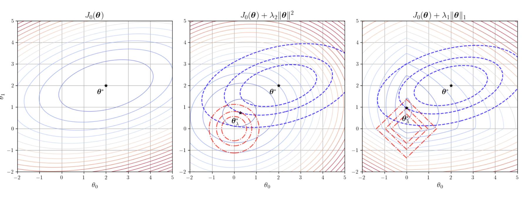
The figure above illustrates the comparison between L1 and L2 regularization constraints.
Kernel Methods
Linear regression can only classify data using a single straight cut, but real-world data is often entangled and cannot be separated by a straight line. To handle complex nonlinear data, we map the original features \(x\) to a higher-dimensional space via a function \(\phi(x)\). The dimensionality of this higher-dimensional space can be extremely high or even infinite (as with the Gaussian kernel), and explicitly computing the coordinates of \(\phi(x)\) would cause computational explosion. The key insight is to use inner products (similarity) to bypass the explicit feature transformation and perform linear operations directly in the high-dimensional space.
The diagram of the mapping function \(\phi(\boldsymbol{x})\) is shown below:
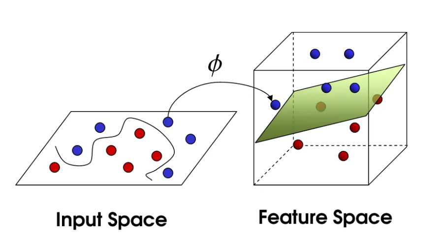
Once the data is lifted to a high-dimensional space, computation becomes prohibitively expensive. If you want to compute the similarity (inner product) of two high-dimensional vectors, you may need thousands of multiplications. Kernel methods were developed as a shortcut. Their essence lies in the ability to compute the inner product of two samples in the high-dimensional space directly through simple operations in the low-dimensional space.
Kernel methods effectively achieve dimensionality lifting through the kernel function \(K(\boldsymbol{x}_i, \boldsymbol{x}_j) = \phi(\boldsymbol{x}_i)^{\text{T}}\phi(\boldsymbol{x}_j)\). Once you define a kernel function, you have implicitly introduced the corresponding mapping \(\phi\). The most fascinating aspect of kernel functions is that some kernels (such as the RBF Gaussian kernel) correspond to mappings of infinite dimensionality. If you tried to manually lift data to infinite dimensions, the computer would simply crash. But the kernel function only needs to compute a simple exponential function \(\exp(-\gamma\|\boldsymbol{x}_i - \boldsymbol{x}_j\|^2)\) to effortlessly perform linear computation in an infinite-dimensional space.
Let us now walk through the derivation of kernel methods.
In linear regression, our goal is to find an optimal parameter \(\boldsymbol{\theta}\). When we introduce \(L_2\) regularization (Ridge Regression), the loss function becomes:
By differentiating and setting the derivative to zero, we obtain the well-known analytical solution:
This formula is based on feature space — if features have \(d\) dimensions, we need to invert a \(d \times d\) matrix. But hidden here is a deep mathematical connection: the optimal weight vector \(\boldsymbol{\theta}\) can actually be expressed as a linear combination of the training samples. That is, \(\boldsymbol{\theta} = \boldsymbol{X}^{\text{T}}\boldsymbol{\alpha}\).
To prove this, we use the matrix identity: \((\boldsymbol{P}\boldsymbol{Q} + \lambda \boldsymbol{I})^{-1}\boldsymbol{P} = \boldsymbol{P}(\boldsymbol{Q}\boldsymbol{P} + \lambda \boldsymbol{I})^{-1}\).
Substituting \(\boldsymbol{P} = \boldsymbol{X}^{\text{T}}\) and \(\boldsymbol{Q} = \boldsymbol{X}\) into the analytical solution, a remarkable transformation occurs:
Notice the rightmost expression. We define \(\boldsymbol{\alpha} = (\boldsymbol{X}\boldsymbol{X}^{\text{T}} + \lambda \boldsymbol{I})^{-1}\boldsymbol{y}\), thus rigorously proving that \(\boldsymbol{\theta} = \boldsymbol{X}^{\text{T}}\boldsymbol{\alpha}\).
When predicting a new sample \(\boldsymbol{x}\), we substitute the new expression for \(\boldsymbol{\theta}\):
Expanding this, it becomes:
This is a fundamental leap: the prediction no longer relies directly on the accumulation of weights, but instead depends on the similarity (inner product) between the new sample \(\boldsymbol{x}\) and each training sample \(\boldsymbol{x}_i\). What was originally linear regression has now become "weighting labels by similarity."
When the linear model cannot fit nonlinear data, we consider mapping the data to a higher-dimensional space \(\phi(\boldsymbol{x})\). Following the logic above, all inner products \(\boldsymbol{x}^{\text{T}}\boldsymbol{x}_i\) become high-dimensional inner products \(\phi(\boldsymbol{x})^{\text{T}}\phi(\boldsymbol{x}_i)\).
But explicitly computing high-dimensional coordinates is extremely expensive, or even impossible (e.g., mapping to infinite dimensions). Thus we introduce the kernel function:
The essence of the kernel trick is: we directly define the computation rule for the inner product without needing to know the coordinates after mapping. For example, the Gaussian kernel (RBF) directly computes high-dimensional similarity in low-dimensional space, giving the model the ability to handle extremely complex decision boundaries.
With this, we complete the full evolution from ordinary linear regression to kernel methods. We define the kernel matrix \(\boldsymbol{K}\)* where *\(K_{ij} = K(\boldsymbol{x}_i, \boldsymbol{x}_j)\).
Training phase: Instead of solving for the feature weights \(\boldsymbol{\theta}\), we solve for the sample weight coefficients \(\boldsymbol{\alpha}\):
Prediction phase: For a new sample \(\boldsymbol{x}\), we compute its similarity with all training samples via the kernel function, then take a weighted sum to produce the result:
Kernel methods, through "reconstructing the analytical solution," transform the dependence on features into a dependence on pairwise inner products between samples. This allows us to leverage the powerful fitting capability of high-dimensional spaces while cleverly circumventing their computational cost.
Hyperparameters and Validation Sets
We have already seen that a model's weights are iteratively optimized during training on the dataset. In addition, there are certain hyperparameters that are manually set in advance and remain fixed throughout training.
Hyperparameters are not learned by the learning algorithm itself from the training set. If hyperparameters were optimized on the training set, the algorithm would always tend to select the maximum possible model capacity, leading to severe overfitting. Therefore, we need to construct a validation set.
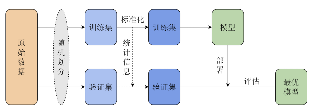
The most common approach is to split the original training data into two parts:
- Training set (approximately 80%): used for learning regular parameters (weights).
- Validation set (approximately 20%): used for estimating generalization error and tuning/selecting hyperparameters accordingly.
Because we select hyperparameters based on validation set performance, the error on the validation set will be lower than the true generalization error. After all hyperparameter optimization is complete, a test set must be used for a fair assessment of model performance.
When you introduce \(L_2\) regularization (Ridge Regression) to prevent overfitting, you introduce one of the most important hyperparameters: the regularization coefficient \(\lambda\)*. If you do not use the analytical solution but instead use *gradient descent to solve for \(\boldsymbol{\theta}\), you will encounter hyperparameters that control the training process: learning rate, number of epochs, and batch size.
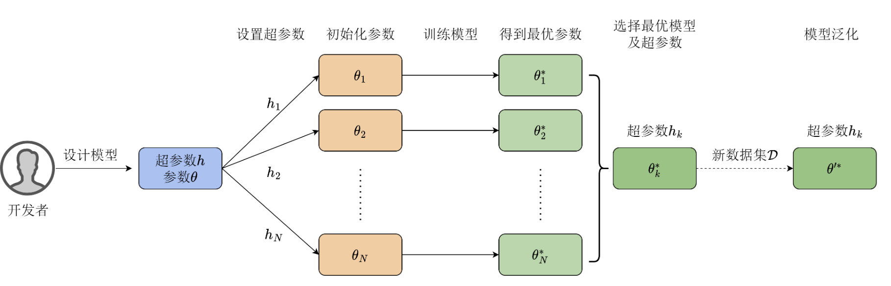
Since hyperparameters cannot be automatically updated, developers must find optimal values through experimentation, a process known as tuning. The tuning process relies heavily on experience:
- Repeated experiments: Specify a set of hyperparameters, train the model, and observe validation set performance; if results are unsatisfactory, adjust hyperparameters, reinitialize the model, and repeat the optimization process.
- Balancing complexity: The number of hyperparameters affects the time needed to find the optimal model. Too many hyperparameters make tuning extremely difficult.
- Value of experience: Skilled algorithm engineers can quickly narrow down the tuning range based on task characteristics and data distribution.
Although hyperparameters traditionally require manual adjustment, research areas such as Automated Machine Learning (AutoML) aim to have computers automatically optimize model architecture and hyperparameters, reducing the cost of human intervention.
Cross-Validation
Cross-validation prevents us from being misled by "luck" at the evaluation procedure level. The dataset is randomly split into \(K\) folds, with training and validation performed in rotation, and the average error taken at the end. This ensures that the hyperparameters we select perform robustly across the "entire book," rather than happening to score well on a few specific questions (validation set), thereby preventing overfitting.
Model Selection
- NFL tells us: there is no invincible algorithm — we must choose models based on the problem.
- i.i.d. tells us: as long as training and testing environments are consistent, learning has mathematical guarantees.
- Model selection tells us: we must find a balance between fitting ability and stability.
No Free Lunch Theorem
The NFL theorem mathematically defines the boundaries of learning.
Suppose we have an algorithm \(a\). We train it on dataset \(\mathcal{D}\) to obtain a hypothesis \(h = a(\mathcal{D})\). We want to know its error on the test set (unseen data).
The NFL theorem states that if we average over all possible target functions \(f\) (i.e., all possible patterns):
Whether your algorithm is a "deep neural network" or "coin flipping," the aggregate score across all possible problems is the same. So why do algorithms differ in practice? Because real-world patterns constitute only a tiny fraction of "all possible patterns." Machine learning is not "alchemy" — it must rely on inductive bias. That is, you must first assume the world has some kind of regularity (e.g., smoothness, periodicity) for your algorithm to be effective.
Independent and Identically Distributed (i.i.d.)
Since NFL says there is no universal algorithm, we must impose constraints on the data for learning to be meaningful. i.i.d. is the most fundamental constraint.
Assume a dataset \(\mathcal{D} = \{(x_1, y_1), \dots, (x_m, y_m)\}\).
Independence:
This means samples do not interfere with each other. Drawing the first person's height does not affect drawing the second person's height.
Identically Distributed:
This means the training set and test set are drawn from the same bag.
By the Law of Large Numbers, when the sample size \(m\) is sufficiently large, the average error computed on the training set (empirical risk) converges to the expected error over the entire distribution (expected risk):
Without i.i.d., there is no necessary mathematical connection between training error and test error, and learning becomes mere guessing.
Bias-Variance Decomposition
With i.i.d. guaranteeing that "learning is feasible," we must face the challenge posed by NFL: which model to choose? The core mathematical framework here is Bias-Variance Decomposition.
For a test point \(x\), our predicted value is \(\hat{f}(x)\) and the true value is \(y\) (which includes noise \(\epsilon\)). The expected error can be decomposed as:
Through algebraic manipulation, it decomposes into three components:
- \(\text{Bias}^2\) (Squared Bias): \((\mathbb{E}[\hat{f}(x)] - f(x))^2\)
- Measures: the gap between the model's average prediction and the true value.
- Represents: the model's fitting ability.
- \(\text{Variance}\): \(\mathbb{E}\left[(\hat{f}(x) - \mathbb{E}[\hat{f}(x)])^2\right]\)
- Measures: the fluctuation of the model's performance across different training sets.
- Represents: the model's stability.
- \(\sigma^2\) (Irreducible Error): Noise.
The essence of model selection is to find a model that minimizes the sum of \(\text{Bias}^2 + \text{Variance}\), given the scale and complexity of the data.
- Simple models (e.g., linear regression): High bias, low variance. The model is too rigid and cannot learn complex patterns (underfitting).
- Complex models (e.g., deep neural networks): Low bias, high variance. The model is too sensitive and even learns the noise in the training set (overfitting).
Classification Tasks
Logistic Regression is a classification algorithm, not a regression algorithm. All prediction results are assigned to a binary classification, such as +1 and -1. We use logistic regression as an example to explain classification tasks and related key concepts.
Sigmoid
The idea behind logistic regression is quite clever:
- Use a linear regression model to compute a score
- The higher this score, the more the model believes the sample belongs to the +1 class; the lower the score, the more it leans toward the -1 class. A score of 0 means the model is undecided, sitting on the decision boundary.
- We use the Sigmoid function (also called the Logistic function) to squash this arbitrarily large score into the (0,1) interval, making it a valid probability value:
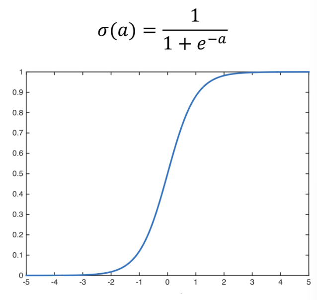
The figure above shows the Sigmoid function and its graph.
Softmax
If we replace Sigmoid with Softmax, we obtain multi-class logistic regression:
The formula above maps a real-valued vector \([a_1, a_2, \ldots, a_K]\) to a probability distribution:
Its key properties include: each output value lies in the (0,1) interval, and all output values sum to 1. It is commonly used in classification models and as the output layer of multi-class neural networks.
Any artificial neural network can append Softmax after a linear layer (regression layer) to output probabilities, thereby performing classification. For example, suppose we want to determine whether an image contains a cat, a dog, or a pig, and the model outputs: cat(2.0), dog(1.0), pig(0.1). These raw scores are difficult to interpret intuitively. The Softmax function compresses these scores to the (0, 1) range while ensuring that the probabilities across all classes sum to 1.
Maximum Likelihood Estimation
First, let us introduce a mathematical concept: likelihood.
"Probability" predicts results given known parameters, while "likelihood" infers parameters given observed results.
For example, suppose we have a coin, and we discuss its "heads probability" \(\theta\).
- Probability:
- Premise: I already know the coin is fair (parameter \(\theta = 0.5\) is fixed).
- Question: What is the chance of getting 7 heads in 10 tosses?
- Logic: Parameters \(\to\) data (predicting the future).
- Likelihood:
- Premise: I do not know whether the coin is fair (parameter \(\theta\) is unknown), but I have already tossed it 10 times and observed 7 heads (data is fixed).
- Question: Given this outcome, is it more plausible that the coin is fair (\(\theta = 0.5\)) or loaded (\(\theta = 0.7\))?
- Logic: Data \(\to\) parameters (reverse-engineering the truth).
Although likelihood and probability sound similar in everyday language, in formulae they actually use the same function, just with different variables:
- When you fix the parameter \(\theta\) and vary the data \(X\), it is the probability function.
- When you fix the observed data \(X\) and vary the parameter \(\theta\), it is the likelihood function.
When constructing the mathematical framework for logistic regression, defining the optimization objective is a crucial step. For probabilistic models, we typically adopt the Maximum Likelihood Estimation (MLE) framework, whose core idea is to find a set of parameters \(\theta\) that maximizes the probability of the model correctly predicting the labels in the training data.
Specifically, let there be \(N\) samples \(\boldsymbol{x}_1, \dots, \boldsymbol{x}_N\) with classes \(y_1, \dots, y_N\). For each sample \(\boldsymbol{x}_i\), when \(y_i = 0\), the probability of a correct prediction is \(1 - f_{\theta}(\boldsymbol{x}_i)\); when \(y_i = 1\), it is \(f_{\theta}(\boldsymbol{x}_i)\). To unify both cases, the probability of correctly predicting a single sample is \(f_{\theta}(\boldsymbol{x}_i)^{y_i}(1 - f_{\theta}(\boldsymbol{x}_i))^{1-y_i}\). Assuming samples are pairwise independent, the total probability of correctly classifying all samples is the likelihood function:
To simplify computation and avoid floating-point underflow issues that arise when computers handle products of many small numbers, we typically take the logarithm of the likelihood function to obtain the log-likelihood, converting the product into a sum:
Since the logarithm is a monotonically increasing function, optimizing \(l(\theta)\) yields the same parameters as optimizing \(L(\theta)\). Therefore, our optimization objective is formally \(\max_{\theta} l(\theta)\).
To find the parameters that maximize \(l(\theta)\), we compute its gradient. Using the derivative properties of the Sigmoid function, the gradient of \(l(\theta)\) is:
Substituting \(f_{\theta}(\boldsymbol{x}) = \sigma(\boldsymbol{\theta}^{\text{T}}\boldsymbol{x})\) and using \(\nabla_{\theta}\sigma(\boldsymbol{\theta}^{\text{T}}\boldsymbol{x}) = \sigma(\boldsymbol{\theta}^{\text{T}}\boldsymbol{x})(1 - \sigma(\boldsymbol{\theta}^{\text{T}}\boldsymbol{x}))\boldsymbol{x}\), the gradient simplifies to a remarkably clean form:
By convention, we convert the optimization objective to minimizing the loss function \(J(\theta) = -l(\theta)\). According to the gradient descent algorithm, with learning rate \(\eta\), the update rule for \(\theta\) is:
In engineering practice, to eliminate the effect of sample size on the learning rate and improve computational efficiency, we typically average over samples and define the sample matrix \(\boldsymbol{X} = (\boldsymbol{x}_1, \dots, \boldsymbol{x}_N)^{\text{T}}\) and label vector \(\boldsymbol{y} = (y_1, \dots, y_N)^{\text{T}}\). The gradient in matrix form is then \(\nabla J(\theta) = -\nabla l(\theta) = \boldsymbol{X}^{\text{T}}(\sigma(\boldsymbol{X}\theta) - \boldsymbol{y})\), and the corresponding parameter update in matrix form becomes:
To further improve the model's generalization ability, we add an \(L_2\) regularization constraint. With regularization coefficient \(\lambda\), the complete optimization objective and update formulas become:
The loss function of logistic regression is convex, meaning that regardless of the initial parameters, the gradient descent trajectory will ultimately converge to the optimal solution \(\theta^*\).
When facing multi-class tasks, logistic regression must be extended to Softmax Regression. We use the softmax function to map the linear prediction \(\boldsymbol{\theta}^{\text{T}}\boldsymbol{x}\) to multi-class probabilities, defined as:
Here \(z\) is a \(K\)-dimensional score vector, where each dimension \(z_j \in (-\infty, +\infty)\) represents the score for class \(j\). The Softmax function maps scores to the \((0, 1)\) interval while ensuring all class probabilities sum to 1, making it interpretable as a probability distribution over a discrete random variable.
It is worth noting that the Softmax function preserves the original ordering of scores and avoids the non-differentiability problem of hard max through the exponential operation. In fact, when the number of classes \(K=2\), the Softmax function reduces to the logistic regression function. In other words, logistic regression is simply a special case of the Softmax function under the binary classification setting.
Cross-Entropy Loss Function
Based on the principle of maximum likelihood estimation, we use the cross-entropy loss function as the loss function for logistic regression.
In classification tasks, the model's output is no longer a specific value like "monthly salary of 20k," but rather a probability (e.g., 80% chance it's a cat).
- Ground truth (\(y\)): Typically a "one-hot" vector. For example, if it truly is a cat, then \([1, 0]\).
- Model prediction (\(\hat{y}\)): A probability distribution. For example, the model says the probability of being a cat is \([0.8, 0.2]\).
The task of cross-entropy is to measure the "distance" between these two probability distributions. The more accurate the prediction, the smaller the cross-entropy; the more off the prediction, the larger the cross-entropy.
The Cross-Entropy Loss function is as follows:
where \(y\) is the true label and \(\hat{y}\) is the predicted probability. Its mechanism works as follows:
Suppose we want to compute a classification judgment on whether "a programmer gets a job offer." The specific meaning in the formula is:
MSE computes the physical distance between predicted and true values, while cross-entropy computes the information divergence between the predicted probability and the true distribution. The reason for using cross-entropy loss as the loss function for classification tasks instead of MSE is that when predictions are egregiously wrong, MSE can only approach 1 at most, whereas cross-entropy can drive the loss to very large values, compelling the model to make larger adjustments in the correct direction during parameter updates.
Evaluation Metrics
In machine learning classification problems, evaluating model quality by looking solely at "accuracy" is insufficient. Depending on data distribution (whether balanced or not) and business tolerance for different types of errors, we need to evaluate from multiple dimensions.
Before discussing specific metrics, we must understand the confusion matrix. It records the alignment between model predictions and true values:
- TP (True Positive): Predicted positive, actually positive.
- TN (True Negative): Predicted negative, actually negative.
- FP (False Positive): False alarm — predicted positive, actually negative.
- FN (False Negative): Miss — predicted negative, actually positive.
The most commonly used core metrics include:
(1) Accuracy represents the proportion of correctly predicted samples out of all samples, and is the most intuitive metric:
However, with imbalanced classes (e.g., 99% of samples are negative), accuracy can be seriously misleading, which is why precision and recall are needed.
(2) Precision (also called positive predictive value) represents the proportion of truly positive samples among all samples predicted as positive. It is suitable for scenarios sensitive to "false alarms," such as spam filtering, where extremely high precision is needed to avoid misclassifying legitimate emails:
(3) Recall (also called sensitivity or true positive rate) represents the proportion of actual positive samples that were correctly identified by the model. It is suitable for scenarios sensitive to "misses," such as cancer detection or earthquake early warning, where the goal is to catch as many positive cases as possible:
(4) F1-Score is the harmonic mean of precision and recall. Since the two are often in conflict (trade-off), the F1 score provides a balanced reference criterion:
(5) ROC Curve and AUC provide a higher-dimensional evaluation. The ROC curve plots the False Positive Rate (FPR) on the x-axis and the True Positive Rate (TPR) on the y-axis, reflecting model performance across different thresholds. AUC is the area under the curve — the closer to 1, the stronger the model's classification ability. This metric is insensitive to class imbalance.
(6) PR Curve (Precision-Recall Curve) plots recall on the x-axis and precision on the y-axis. When there is severe class imbalance (very few positive samples), the PR curve typically reflects model performance more faithfully than the ROC curve.
Case Study
Let us look at a concrete example and demonstrate how to apply the formulas discussed above.
Consider the following scenario: predicting a programmer's "interview outcome."
The three features (independent variables) we observe are:
- \(x_1\): Number of coding problems solved (e.g., 500 problems)
- \(x_2\): Project experience (e.g., 3 projects)
- \(x_3\): Years of experience (e.g., 5 years)
Each feature has a corresponding weight (\(w\)), plus an intercept (\(b\)).
Suppose the model has learned the parameters: \(w_1=0.1, w_2=2, w_3=1, b=-10\).
Using linear regression, we plug in the programmer's feature values to get the prediction:
That is, the predicted interview score for this candidate is 51.
Logistic regression takes the linear regression result and transforms it into a function bounded between 0 and 1. Assume there are only two outcomes: getting an Offer (\(1\)) or being rejected (\(0\)). We feed the raw score \(z=51\) from the linear regression into the Sigmoid function:
Since \(51\) is very large, \(e^{-51}\) approaches \(0\). The probability of getting an offer is approximately 99.9%. From a classification perspective, the predicted outcome is: gets the offer.
Softmax can handle multi-class problems. For example, suppose after the programmer gets an offer, we need to determine the job level: Junior, Mid-level, or Senior.
In this case, the model has three separate sets of parameters (one scoring criterion for each level):
- \(z_{\text{Junior}} = 10\) (low score)
- \(z_{\text{Mid}} = 30\) (medium score)
- \(z_{\text{Senior}} = 51\) (the high score computed earlier)
Since \(e^{51}\) is far larger than the other terms, the model is nearly 100% certain this person should be classified as Senior.
In reality, you observe that this candidate (500 problems / 3 projects / 5 years) received a rejection (\(y=0\)). But the model calculated \(P(Offer) = 0.999\). The model predicted a near-certain offer, yet the person was rejected. This indicates that the \(w\) and \(b\) values are incorrect.
Since the ground truth is "rejected," the probability of "rejected" is \(1 - 0.999 = 0.001\). MLE's objective is to increase this probability of the actually observed outcome (\(0.001\)). To increase \(0.001\), the algorithm adjusts the parameters so that the next time the model computes \(z\), it will be smaller and \(P(Offer)\) will decrease. When the model parameters make the probability of "rejection" look reasonable (e.g., \(0.9\)), MLE has succeeded. Gradient descent forces \(w_1, w_2, w_3\) to decrease, or pushes \(b\) more negative (e.g., \(b = -100\)).
Summary of Common Supervised Learning Algorithms/Models
Below is a list of common algorithms with brief descriptions of their loss functions and basic approaches to finding optimal parameters. For detailed coverage of specific models, please refer to the corresponding chapter notes.
Generalized Linear Models
The Generalized Linear Model (GLM) is a flexible extension of linear regression. Ordinary linear regression requires that the data follow a normal distribution and that the relationship between independent and dependent variables be linear. However, in the real world, much data does not conform to these assumptions (e.g., whether an email is spam, the number of accidents at an intersection). GLMs were designed to handle such "irregular" data.
Linear regression, logistic regression, and others all fall under generalized linear models.
Linear Regression
Logistic Regression
Bilinear Models
Suppose we have two vector inputs \(\mathbf{x} \in \mathbb{R}^m\) and \(\mathbf{y} \in \mathbb{R}^n\). A standard bilinear mapping can be expressed as:
where \(\mathbf{W} \in \mathbb{R}^{m \times n}\) is a weight matrix.
- Linearity: If \(\mathbf{y}\) is fixed, the function is linear in \(\mathbf{x}\); if \(\mathbf{x}\) is fixed, the function is linear in \(\mathbf{y}\).
- Interaction terms: When expanded, it computes the weighted sum of all possible \(x_i y_j\) products.
Ordinary linear models (e.g., \(y = w_1x_1 + w_2x_2\)) assume variables are independent. In reality, however, many factors are interrelated. In computer vision, the seminal "bilinear models" paper (Tenenbaum & Freeman) proposed:
- Factor A: The content of a letter (e.g., whether it is 'A' or 'B').
- Factor B: The font style of the letter (e.g., italic or bold). The final generated image is the "product" effect of these two factors. Simple linear addition (style + content) cannot perfectly reconstruct such complex transformations.
Common application scenarios also include:
- Matrix Factorization: A user's interest vector is \(\mathbf{u}\), an item's feature vector is \(\mathbf{v}\), and the predicted rating is \(r = \mathbf{u}^\top \mathbf{v}\).
- In deep learning (especially fine-grained image classification), bilinear pooling is used to capture spatial correlations between different channels in feature maps. It computes the outer product of feature vectors at each pixel: \(\mathbf{z} = \mathbf{f} \mathbf{f}^\top\). This helps the model recognize very subtle features, such as specific textures in bird feathers.
- In early relation extraction or semantic parsing, bilinear transformations were commonly used to measure certain relationships between two entities (subject and object).
KNN Algorithm
The KNN algorithm is one of the most introductory machine learning algorithms, with a remarkably simple principle. We start with KNN and progressively learn various machine learning algorithms. Neural network-based algorithms are collectively referred to as deep learning algorithms; see the deep learning chapter.
KNN (K-Nearest Neighbors) can be used for both classification and regression tasks.
The core logic of KNN is to assign the current sample to the majority class among its neighbors. The value of \(K\) is critical:
- \(K\) too small: The classification result is easily affected by individual noisy data points near the target sample.
- \(K\) too large: Distant, irrelevant samples may be included. Therefore, \(K\) should be dynamically adjusted based on the dataset.
KNN can be used for both regression and classification.
For classification tasks, let the set of labeled samples be \(\boldsymbol{x}_0\). For an unlabeled sample \(\boldsymbol{x}\), define its neighborhood \(N_K(\boldsymbol{x})\) as the set of \(K\) samples \(\boldsymbol{x}_1, \boldsymbol{x}_2, \dots, \boldsymbol{x}_K\) from \(\boldsymbol{x}_0\) closest to \(\boldsymbol{x}\). Their corresponding classes are \(y_1, y_2, \dots, y_K\). Count the number of samples in \(N_K(\boldsymbol{x})\) belonging to class \(j\), denoted as \(G_j(\boldsymbol{x})\):
where \(\mathbb{I}(p)\) is the indicator function, equal to \(1\) when \(p\) is true and \(0\) otherwise. The class \(\hat{y}(\boldsymbol{x})\) of \(\boldsymbol{x}\) is the class that maximizes \(G_j(\boldsymbol{x})\):
For regression tasks, given a sample \(\boldsymbol{x}\), we predict its corresponding real value \(y\). KNN considers the \(K\) neighbor points \(\boldsymbol{x}_i \in N_K(\boldsymbol{x})\) and computes the weighted average of their corresponding values \(y_i\) to obtain the prediction \(\hat{y}(\boldsymbol{x})\):
The weights \(w_i\) represent the importance of each neighbor. Common weight assignment methods include:
- Setting all \(w_i = \frac{1}{K}\) (simple average).
- Setting weights inversely proportional to distance.
- Learning the weights as model parameters.
Let us look at a KNN regression example — color transfer.
We know that RGB records the color information of the three primary colors. Computers also use LAB to represent colors, where L represents lightness, A represents the red-green component, and B represents the yellow-blue component. In short, LAB primarily records lightness, designed to simulate human perception.
We can use LAB to perform color transfer. Suppose we have a grayscale image A and a color image B. Image A's LAB information only contains L without AB; image B has complete LAB information. We can use the mapping relationship between L and AB color channels in B to colorize A.
In this process, L is the input X and AB is the output Y. By feeding the LAB information into the model, we can train the mapping relationship between L and AB. On this basis, every L value will correspond to an AB value.
We can use sklearn for a quick training:
knn = KNeighborsRegressor(n_neighbors=25, weights='distance', n_jobs=-1)
knn.fit(X_train, y_train)
Specifically, for a point x in the grayscale image with lightness L=50, we search among the tens of thousands of pixels in the color image for those with lightness closest to 50, select 25 of them, and average their colors as the prediction for point x. The weight='distance' parameter means pixels with closer colors have more influence — that is, the colors of these 25 pixels are not simply averaged equally.
Naive Bayes
- Loss function: No explicit loss function.
- It is a generative model whose goal is to maximize the posterior probability \(P(Y|X)\).
- Parameter estimation: Counting and frequency estimation.
- Parameter estimation amounts to computing empirical estimates of prior and conditional probabilities (i.e., counting from a lookup table). To prevent zero probabilities, Laplace Smoothing is typically applied.
SVM
- Loss function: Hinge Loss + \(L_2\) regularization term.
- Formula: \(L(w, b) = \sum \max(0, 1 - y_i(w^Tx_i + b)) + \lambda ||w||^2\).
- Parameter optimization: Quadratic Programming (QP).
- Typically transformed into the dual problem and solved iteratively using the SMO algorithm (Sequential Minimal Optimization) for the Lagrange multipliers.
Decision Tree
Decision trees are an intuitive and powerful supervised learning algorithm, applicable to both classification and regression. The core idea is to recursively partition the data space into sub-regions through a series of if-else decisions, forming a tree structure. The greatest advantage of decision trees is their high interpretability — you can clearly see the rationale behind each decision made by the model.
Splitting Criteria
At each node, a decision tree must select a feature and a threshold for splitting. The selection criterion is the split that produces the greatest decrease in "impurity" in the child nodes. Different impurity measures give rise to different decision tree algorithms.
(1) Information Gain — ID3 Algorithm
Information gain is based on the concept of entropy. For a dataset \(S\) containing \(K\) classes, the entropy is defined as:
where \(p_k\) is the proportion of class \(k\) samples in \(S\). Higher entropy means more "disorder"; an entropy of 0 indicates complete purity (only one class).
The information gain from splitting dataset \(S\) on feature \(A\) is:
The ID3 algorithm selects the feature with the highest information gain at each split. However, information gain has a flaw: it favors features with many distinct values (in the extreme case, using "ID" as a feature gives one branch per sample — maximum information gain but zero generalization).
(2) Gain Ratio — C4.5 Algorithm
C4.5 penalizes features with too many values by introducing Split Information:
where \(H_A(S) = -\sum_{v} \frac{|S_v|}{|S|} \log_2 \frac{|S_v|}{|S|}\) is the intrinsic entropy of feature \(A\). Features with more values yield a larger \(H_A(S)\), thereby penalizing the bias of information gain.
(3) Gini Impurity — CART Algorithm
CART (Classification and Regression Tree) uses Gini impurity as its measure:
The intuitive meaning of the Gini impurity is: the probability that two randomly drawn samples from the dataset belong to different classes. A smaller Gini impurity indicates higher dataset purity.
CART is the most commonly used decision tree algorithm today (Scikit-learn uses CART by default). Unlike the multi-way trees of ID3/C4.5, CART builds binary trees — each split produces exactly two child nodes.
(4) Splitting Criterion for Regression Trees
For regression tasks, CART uses Mean Squared Error (MSE) as the splitting criterion. For the sample set \(S_t\) in node \(t\), its MSE is:
where \(\bar{y}_t\) is the mean target value of all samples in node \(t\). The feature and threshold that yield the greatest reduction in weighted MSE are selected.
Pruning
If a decision tree is allowed to grow freely, it will keep splitting until each leaf node contains only a single sample, inevitably leading to severe overfitting. Pruning is the core mechanism for controlling decision tree complexity.
- Pre-pruning: Stops tree growth early during construction. Common conditions include:
* Setting maximum depth (
max_depth) * Setting minimum samples per leaf node (min_samples_leaf) * Setting minimum samples required for a split (min_samples_split) * Setting a minimum impurity decrease threshold
- Post-pruning: Lets the tree grow fully, then prunes from the bottom up by removing subtrees that contribute little to validation set performance. CART uses Cost-Complexity Pruning, with the objective function:
where \(|T|\) is the number of leaf nodes and \(\alpha\) is the regularization parameter. A larger \(\alpha\) leads to more aggressive pruning and a simpler tree.
Advantages and Disadvantages of Decision Trees
| Advantages | Disadvantages |
|---|---|
| Highly interpretable, can be visualized | Prone to overfitting (requires pruning) |
| No feature standardization needed | Sensitive to small data changes (high variance) |
| Handles both numerical and categorical features | Decision boundaries are axis-aligned (poor at capturing diagonal relationships) |
| Can automatically handle missing values (CART) | Greedy algorithm, cannot guarantee global optimality |
The high variance problem of decision trees — small changes in training data can lead to completely different tree structures — is the core issue that ensemble methods (Random Forest, Gradient Boosting) aim to solve.
Ensemble Learning
The core idea of ensemble learning is "the wisdom of the crowd" — combining multiple weak learners into a single strong learner. Based on different combination strategies, ensemble learning is divided into two main schools:
| School | Core Idea | Base Learner Relationship | Representative Algorithms |
|---|---|---|---|
| Bagging | Parallel training, voting/averaging | Independent, parallel | Random Forest |
| Boosting | Sequential training, progressive correction | Dependent, sequential | AdaBoost, GBDT, XGBoost, LightGBM |
Random Forest
Random Forest combines the Bagging idea with decision trees. Proposed by Leo Breiman in 2001, it reduces model variance by constructing a large number of decision trees and aggregating their predictions.
Core mechanism:
- Bootstrap sampling: Draw \(N\) samples with replacement from the original dataset (approximately 63.2% of original samples are selected; the remainder are called OOB (Out-of-Bag) samples)
- Random feature subsets: At each node split, instead of using all \(d\) features, randomly select \(m\) features (typically \(m = \sqrt{d}\) for classification, \(m = d/3\) for regression)
- Independent growth: Each tree grows without pruning to maximum depth
- Aggregated prediction: Majority voting for classification, averaging for regression
Why does Random Forest work?
Let the variance of a single tree be \(\sigma^2\) and the correlation between trees be \(\rho\). The variance of the ensemble of \(n\) trees is:
Random Forest reduces \(\rho\) (inter-tree correlation) through two layers of randomness: sample randomness and feature randomness. When \(\rho\) is small, increasing the number of trees \(n\) effectively reduces the second term, thereby lowering overall variance. This is why Random Forest almost never overfits — adding more trees only continues to decrease (or plateau) the variance, never making it worse.
OOB evaluation: Each tree's OOB samples can be used to evaluate that tree's generalization performance. Aggregating OOB evaluation results across all trees yields an unbiased estimate of the entire model's performance, without needing a separate validation set.
Practical considerations:
- Random Forest is insensitive to hyperparameters; default settings usually yield good results
- OOB error and feature importance can assist with feature selection
- Naturally supports parallel computation (each tree is built independently)
- Remains a very strong baseline for classification and regression tasks on tabular data
Gradient Boosting Decision Tree (GBDT)
GBDT is the flagship of the Boosting school, proposed by Jerome Friedman in 1999. Unlike Bagging, which builds weak learners in parallel, Boosting is sequential — each new tree attempts to correct the collective errors of all preceding trees.
Core idea:
GBDT views the optimization process as gradient descent in function space. Let the current model be \(F_{t-1}(x)\); the \(t\)-th tree \(f_t(x)\) fits the negative gradient of the loss function with respect to the current model's predictions:
When the loss function is MSE, the negative gradient is exactly the residual \(y_i - F_{t-1}(x_i)\), which is the intuitive origin of the name "gradient boosting."
The update process is:
where \(\eta\) is the learning rate (shrinkage), typically set to a small value (e.g., 0.01--0.1). A smaller learning rate combined with more trees yields better results but requires longer training time.
XGBoost
XGBoost (eXtreme Gradient Boosting), proposed by Tianqi Chen in 2016, is an efficient engineering implementation and algorithmic improvement of GBDT. XGBoost has shone in Kaggle competitions and remains one of the most widely used models for tabular data in both competitions and industrial applications.
Core improvements over GBDT:
(1) Second-order Taylor expansion
GBDT uses only the first-order derivative (gradient) of the loss function, while XGBoost uses both the first-order derivative \(g_i\) and second-order derivative \(h_i\), performing a second-order Taylor expansion of the loss function:
where:
- \(g_i = \frac{\partial L(y_i, \hat{y}_i^{(t-1)})}{\partial \hat{y}_i^{(t-1)}}\) is the first-order derivative of the loss with respect to the prediction
- \(h_i = \frac{\partial^2 L(y_i, \hat{y}_i^{(t-1)})}{\partial (\hat{y}_i^{(t-1)})^2}\) is the second-order derivative of the loss with respect to the prediction
The second-order information provides curvature information about the loss surface, analogous to the advantage of Newton's method over gradient descent, making each update step more precise and convergence faster.
(2) Regularization term
XGBoost explicitly adds tree complexity penalties to the objective function:
where \(T\) is the number of leaf nodes and \(w_j\) is the weight of the \(j\)-th leaf node. \(\gamma\) penalizes the number of leaf nodes (encouraging simpler trees), and \(\lambda\) is the L2 regularization coefficient (constraining leaf weight magnitudes).
(3) Optimal leaf node weights
By differentiating the objective function with respect to leaf weight \(w_j\) and setting it to zero, we obtain the optimal weight for each leaf node:
and the corresponding contribution of that leaf to the objective function (used to evaluate split gain):
(4) Split gain
XGBoost decides whether to split by comparing the objective function values before and after the split:
A split is performed only when Gain > 0. \(\gamma\) acts as a pre-pruning mechanism.
(5) Engineering optimizations
- Column subsampling: Similar to Random Forest's feature randomness, further reducing overfitting
- Missing value handling: Automatically learns whether missing values should go to the left or right subtree
- Weighted quantile sketch: An approximate algorithm for handling large-scale data
- Cache optimization and parallel computation: Pre-sorted features enable parallel computation of optimal split points for each feature
LightGBM
LightGBM, proposed by Microsoft in 2017, is a strong competitor to XGBoost. While maintaining accuracy, it is typically several times to tens of times faster than XGBoost in training, especially with large datasets and high-dimensional features.
Core innovations:
(1) Histogram-based splitting
XGBoost uses pre-sorted methods to traverse all feature values to find the best split point, with time complexity \(O(\text{data} \times \text{features})\). LightGBM bins continuous feature values (typically 256 bins) and only searches for split points at bin boundaries:
- Time complexity drops to \(O(\text{bins} \times \text{features})\), where bins << data
- Memory consumption shifts from storing each sample's feature value to storing bin indices (uint8), drastically reducing memory usage
- Histogram subtraction acceleration: subtracting one child node's histogram from the parent's yields the other child's histogram
(2) GOSS (Gradient-based One-Side Sampling)
In GBDT, samples with large gradients contribute more to information gain. GOSS retains all samples with large gradients (top \(a\)%) and randomly samples only a portion (\(b\)%) of small-gradient samples, with weight compensation for the sampled small-gradient samples. This significantly reduces computation while preserving key information.
(3) EFB (Exclusive Feature Bundling)
In high-dimensional sparse data (e.g., after one-hot encoding), many features are mutually exclusive (they never take non-zero values simultaneously). EFB bundles these exclusive features into a single feature, effectively reducing feature dimensionality. This optimization is particularly impactful for datasets with many sparse features.
(4) Leaf-wise growth strategy
| Strategy | Description | Characteristics |
|---|---|---|
| Level-wise (XGBoost default) | Grows level by level, splitting all nodes at the same depth | More balanced, less prone to overfitting, but less efficient |
| Leaf-wise (LightGBM default) | Selects the leaf with the highest gain for splitting each time | More efficient, lower loss for the same number of leaf nodes, but requires limiting max_depth to prevent overfitting |
CatBoost
CatBoost, proposed by Yandex in 2017, stands out for its native support of categorical features.
- Ordered Target Encoding: Uses permutation order to compute categorical feature encodings, avoiding the data leakage problem of traditional target encoding
- Ordered Boosting: Uses random permutations during training to avoid prediction shift
- Symmetric Tree: Builds fully symmetric decision trees, which are conducive to GPU acceleration
XGBoost vs LightGBM vs CatBoost Comparison
| Feature | XGBoost | LightGBM | CatBoost |
|---|---|---|---|
| Splitting strategy | Level-wise | Leaf-wise | Symmetric Tree |
| Split search | Pre-sorted / Histogram | Histogram | Histogram |
| Training speed | Moderate | Fast | Moderate |
| Categorical features | Requires manual encoding | Limited support | Native support |
| Missing values | Auto-handled | Auto-handled | Auto-handled |
| GPU support | Supported | Supported | Supported (well-optimized) |
| Best scenario | General purpose | Large data, high dimensions | Heavy categorical features |
Practical recommendations:
- For structured/tabular data classification and regression tasks, XGBoost and LightGBM remain the most commonly used models in industry and competitions as of 2024--2025, often outperforming deep learning models in many scenarios
- When data is small (<100k rows), the three models perform similarly; with larger data, LightGBM's speed advantage becomes pronounced
- When there are many categorical features, consider CatBoost first
- In practice, it is advisable to try all three and select the best model via cross-validation