Tree

Tree Structures

Rooted Tree

A Rooted Tree is a special type of tree structure in which one node is explicitly designated as the root. Once the root is determined, all relationships among the other nodes in the tree (such as parent-child, ancestor, descendant, etc.) are uniquely defined. In the context of computer science and data structures, when we refer to a "tree," we almost always mean a rooted tree by default.

Since trees are special cases of graphs, unrooted trees typically come up only when discussing Minimum Spanning Trees (MSTs) in graph theory.

Binary Tree

A Binary Tree is a special tree structure in which each node has at most two children. The child on the left is called the left subtree, and the child on the right is called the right subtree.

Traversal

Due to the special structure of binary trees, there are three unique traversal orderings: preorder traversal, inorder traversal, and postorder traversal.

Preorder Traversal

Preorder traversal is precisely defined as:

\[ \text{Visit root} \rightarrow \text{Traverse left subtree} \rightarrow \text{Traverse right subtree} \]

.

Inorder Traversal

Inorder traversal is precisely defined as:

\[ \text{Traverse left subtree} \rightarrow \text{Visit root} \rightarrow \text{Traverse right subtree} \]

Inorder traversal is therefore unique to binary trees, and it gives rise to the concepts of predecessor and successor. For details on predecessor and successor, see the relevant section on BSTs.

Postorder Traversal

Postorder traversal is precisely defined as:

\[ \text{Traverse left subtree} \rightarrow \text{Traverse right subtree} \rightarrow \text{Visit root} \]

In terms of memory management, this is the safest way to delete or destroy a tree, because it always processes children before their parent. This ensures that by the time a parent node is processed, all of its dependent child nodes have already been cleaned up or freed, thus avoiding dangling pointers.

Postorder traversal is well-suited for scenarios where child node attributes must be computed before being aggregated at the parent (e.g., computing the height, weight, or path of each subtree).

Complete Binary Tree

A Complete Binary Tree is a binary tree in which every level, except possibly the last, is fully filled, and all nodes on the last level are packed as far left as possible. Because there are no gaps, a complete binary tree can be stored compactly in an array without the need for pointers.

With 0-based array indexing:

Parent: \((i-1)//2\)
Left child: \(2i+1\)
Right child: \(2i+2\)

With 1-based array indexing:

Parent: \(i//2\)
Left child: \(2i\)
Right child: \(2i+1\)

The following is a valid complete binary tree:

The following is NOT a complete binary tree (growth starts from the right; the left side of D is empty):

.

Full Binary Tree

A Full Binary Tree is a binary tree in which every level has the maximum number of nodes.

For example:

       A
      /   \
     B     C
    / \    / \
   D  E  F   G

Full Binary Tree ⊂ Complete Binary Tree ⊂ General Binary Tree

BST

A Binary Search Tree (BST) is a special kind of binary tree with the following key properties that make search, insertion, and deletion operations efficient:

For any node in the tree, if its left subtree is non-empty, then all nodes in the left subtree have values less than that node's value.
For any node in the tree, if its right subtree is non-empty, then all nodes in the right subtree have values greater than that node's value.
Both the left and right subtrees of any node must themselves be binary search trees.

In short: left is smaller, right is larger. Consequently, an inorder traversal of a BST yields a sorted sequence in ascending order — this is also a common method for verifying whether a tree is a valid BST.

All basic BST operations (search, insert, delete) have time complexities proportional to the height of the tree:

Operation	Average Time Complexity	Worst-Case Time Complexity
Search	\(O(\log n)\)	\(O(n)\)
Insert	\(O(\log n)\)	\(O(n)\)
Delete	\(O(\log n)\)	\(O(n)\)

The worst case occurs when elements are inserted in ascending or descending order, causing the BST to degenerate into a linked list with height \(n\), resulting in a worst-case time complexity of \(O(n)\).

Predecessor and Successor

Predecessor and Successor are concepts unique to binary trees, both defined in terms of inorder traversal.

After performing an inorder traversal of a binary tree, the predecessor of node \(x\) is the node immediately before \(x\) in the inorder sequence, and the successor of node \(x\) is the node immediately after \(x\) in the inorder sequence.

In a BST, the predecessor is the node with the largest key among all nodes whose keys are less than \(x\)'s key; the successor is the node with the smallest key among all nodes whose keys are greater than \(x\)'s key. For further details, see the sections on BST and BBST.

LCA (Lowest Common Ancestor)

The Lowest Common Ancestor (LCA) is defined as follows: given two nodes \(u\) and \(v\) in a tree, their lowest common ancestor \(LCA(u, v)\) is the node that is an ancestor of both \(u\) and \(v\) and is farthest from the root (i.e., has the greatest depth).

LCA is not a concept exclusive to BSTs — it applies to all rooted trees. However, in a BST, the ordered property makes finding the LCA particularly efficient.

The core idea is: starting from the root, if the two target nodes \(p\) and \(q\) lie in different subtrees (one left, one right) of the current node, then the current node is the LCA. If both are less than the current node, recurse into the left subtree; if both are greater, recurse into the right subtree.

BBST

A BST does not adjust its own structure during construction. Therefore, if sorted data is inserted in order (e.g., \(10, 15, 20\)), the tree degenerates into a linked list:

\[ \begin{array}{c} 10 \\ \backslash \\ 15 \\ \backslash \\ 20 \end{array} \]

In this case, the time complexity of search, insertion, and deletion degrades from the optimal \(O(\log N)\) to the worst-case \(O(N)\).

AVL Tree

An AVL tree maintains balance by checking the balance factor of each node.

Balance Factor (BF) = Height of left subtree - Height of right subtree

For any node in an AVL tree, its balance factor \(BF\) must satisfy:

\[ |BF| \le 1 \quad \text{or} \quad -1 \le BF \le 1 \]

\(BF = 1\): The left subtree is 1 level taller than the right subtree (left-heavy).
\(BF = 0\): The left and right subtrees have equal height.
\(BF = -1\): The right subtree is 1 level taller than the left subtree (right-heavy).

When \(|BF| > 1\), the tree is unbalanced and requires a rotation to restore balance.

Rotations

Rotations are the core mechanism by which AVL trees maintain balance. A rotation only changes the parent-child relationships among a local set of nodes without affecting higher-level connections. There are two primary rotation operations: Right Rotation and Left Rotation.

It is important to note that because rotations only change local relationships without affecting higher-level ones, the entire tree rotates only when the target of the rotation is the root.

Example:

The right side of this tree is too deep, so we rotate at node 7. Since rotation only changes local relationships, we focus on the subtree rooted at node 7:

Here we call the node to be rotated (7) as x:

RightRotate(x):
    y = x.left
    x.left = y.right
    y.right = x

Since y.right does not exist here, the result after rotation is:

      5
     / \
    4   7
   /   / \
  3   (empty) 9

Reconnecting the new local root (5) back to the original tree:

         2
       /  \
      0    5
     / \  / \
   -1  1  4  7
            / \
           3   9

This gives us the tree after rotation.

Four Types of Imbalance

Based on where the imbalance occurs, there are four types. Here \(x\) denotes the nearest ancestor of the inserted/deleted node with \(|BF|>1\).

When the left subtree is too heavy and the imbalance occurs in the left subtree, it is called an LL imbalance, which requires a right rotation:

When the right subtree is too heavy and the imbalance occurs in the right subtree, it is called an RR imbalance, which requires a left rotation:

When the left subtree is too heavy but the imbalance occurs in the right subtree, it is called an LR imbalance, which requires first a left rotation on y, then a right rotation on x:

When the right subtree is too heavy but the imbalance occurs in the left subtree, it is called an RL imbalance, which requires first a right rotation on y, then a left rotation on x:

.

Red-Black Tree

CLRS13

insert, fixup

A red-black tree is a special type of BST, so all BST properties also apply to red-black trees.

Note that in a red-black tree, "leaf nodes" refer to NIL (Null) nodes, also known as sentinel nodes.

A red-black tree must satisfy the following requirements:

Every node is either red or black.
The root is black.
Every NIL node is black.
If a node is red, then both of its children are black.
For any node, all paths from that node to its descendant NIL nodes contain the same number of black nodes. This count is called the node's black-height.

OS-SELECT

A data structure based on a red-black tree (a type of BBST), called an Order-Statistic Tree, stores the size of the subtree at each node as additional information. Using this information, finding the \(k\)-th smallest element (i.e., \(\text{OS-SELECT}\)) can be done in \(O(\log n)\) time.

Logically, OS-SELECT is a classic recursive procedure:

OS-SELECT(x, i):
    r = x.left.size + 1
    if i == r:
        return x
    elif i < r:
        return OS-SELECT(x.left, i)  // recursive call
    else:
        return OS-SELECT(x.right, i - r) // recursive call

Since \(\text{OS-SELECT}\) is a form of tail recursion (each call either returns or makes a single new call to itself at the end), it can be conveniently converted to an iterative implementation — a common approach in CLRS to avoid the risk of stack overflow and function call overhead from deep recursion.

OS-SELECT(T, i):
    x = T.root
    while x != NIL:
        r = x.left.size + 1
        if i == r:
            return x  // found, return
        elif i < r:
            x = x.left  // move to left subtree
        else:
            i = i - r   // update target rank
            x = x.right // move to right subtree
    return NIL

.

Heap

Binary Heap

A binary heap is structurally a complete binary tree and can therefore be stored in an array.

With 0-based array indexing:

Parent: \((i-1)//2\)
Left child: \(2i+1\)
Right child: \(2i+2\)

With 1-based array indexing:

Parent: \(i//2\)
Left child: \(2i\)
Right child: \(2i+1\)

1765170644150

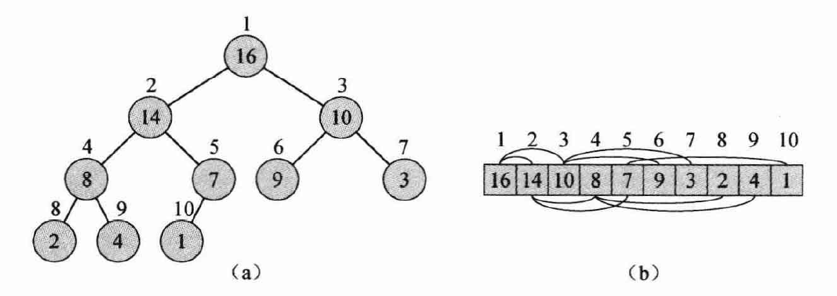
The figure above illustrates both the tree structure and array storage of a binary heap.

A binary heap comes in two variants — Max Heap and Min Heap:

In a max heap, every parent node's value is greater than or equal to the values of its left and right children. The heap top (root) is the largest element in the entire heap.
In a min heap, every parent node's value is less than or equal to the values of its left and right children. The heap top (root) is the smallest element in the entire heap.

The efficiency of a binary heap lies in how it maintains order. We do not need the entire array to be sorted — we only need to maintain the parent-child relationship.

Core Operations

Below we use a min heap as an example to explain the core operations of a binary heap. In Python's implementation, heapq uses a min heap by default; a max heap can be simulated by storing negated values.

(1) Find-Min

This is the simplest operation of a binary heap. By the heap-order property, the root of a min heap is always the smallest element in the entire heap. In the array representation, it is always at index 0.

Complexity: \(O(1)\)

(2) Delete-Min

Remove the root element and restore the heap-order property. This process is accomplished via sift down.

Steps:
1. Remove: Remove the element at index 0 (this is the minimum value to be returned).
2. Replace: Move the last element in the array (the deepest, rightmost leaf node in the heap) to index 0 to fill the vacancy.
3. Compare: Compare the new root with its left and right children.
4. Swap (sift down): If the root is larger than a child, swap it with the smaller child (ensuring the smallest value floats up).
5. Repeat: Repeat steps 3–4 until the node is smaller than both of its children, or it has sunk to a leaf position.
Complexity: \(O(\log n)\). In the worst case, the node sinks from root to leaf, a path whose length equals the tree height.

(3) Decrease-Key

If a node's value decreases, we need to sift it up until the min-heap property is restored.

Prerequisite: You typically need an auxiliary mechanism (such as a hash map) to quickly locate the current index \(i\) of the target element in the heap array.
Steps:
1. Modify: Decrease the value of the element at index \(i\).
2. Check: Because the value decreased, it may now be smaller than its parent, violating the heap-order property.
3. Swap (sift up): If it is smaller than its parent, swap it with the parent.
4. Repeat: Repeat the comparison and swapping until it is larger than its parent, or it has become the root.
Complexity: \(O(\log n)\). The worst case is floating from the bottom to the root.

It is worth noting that we generally only analyze the complexity of Decrease-Key, since Increase-Key is essentially a sift-down operation, which was already covered in Delete-Min above.

(4) Insert

Insert a new element. This is essentially a special case of Decrease-Key (or rather, it relies on the same sift-up mechanism).

Steps:
1. Append: Place the new element at the end of the array (i.e., after the last leaf node in the heap), preserving the complete binary tree shape.
2. Sift up: Perform the same sift-up logic as Decrease-Key — if the new node is smaller than its parent, keep swapping it upward.
Complexity: \(O(\log n)\).

(5) Make-Heap (Build Heap)

Given an unsorted array, transform it into a binary heap that satisfies the heap-order property.

We can build the heap using the MIN-HEAPIFY operation. MIN-HEAPIFY(A, i) assumes that the left and right subtrees of node \(i\) are already valid heaps, but node \(i\) itself may be too large, violating the min-heap property. The goal is to sink \(i\) to the appropriate position. The core idea is:

Assume that node i's left and right subtrees are already heaps, but i is too large and needs to sink.
Find the smallest value among i, i's left child, and i's right child.
If the smallest is not i, swap i with the smallest, then recursively apply MIN-HEAPIFY on the swapped position.

Pseudocode:

MIN-HEAPIFY(A, i)
    l = LEFT(i)
    r = RIGHT(i)
    if l <= A.heap-size and A[l] < A[i]
        smallest = l
    else smallest = i
    if r <= A.heap-size and A[r] < A[smallest]
        smallest = r
    if smallest != i
        exchange A[i] with A[smallest]
        MIN-HEAPIFY(A, smallest)

With the above operation understood, building the heap is straightforward: we apply MIN-HEAPIFY to all non-leaf nodes:

BUILD-MIN-HEAP(A)
    A.heap-size = A.length
    for i = floor(A.length/2) downto 1
        MIN-HEAPIFY(A, i)

The loop starts at floor(A.length/2), which is the last node that has children (i.e., the last non-leaf node). Iterating from here down to 1 (bottom-up) is an absolute prerequisite for the build process to succeed.

Now let us analyze the time complexity. MIN-HEAPIFY is O(log N), and the number of non-leaf nodes is (1/2)N, so it might appear to be O(N log N). However, we must recognize that during the bottom-up traversal, the very first (smallest) sub-heaps processed have very low height but account for half the total nodes! So we need to correctly sum the work at each level:

\[ T(n) = \sum (\text{number of nodes} \times \text{sift-down height}) \]

The total cost formula is:

\[ T(n) = n \times \sum_{h=0}^{\log n} \frac{h}{2^{h+1}} \]

The series on the right converges to 1, therefore:

\[ T(n) = n \times 1 = O(n) \]

This result is very important and should be memorized: The time complexity of building a binary heap is O(n).

(6) Meld (Merge)

Merge two binary heaps \(H_1\) and \(H_2\) into a single new binary heap. This is a weakness of binary heaps. Because a binary heap is a compact array structure, you cannot simply merge them by rearranging pointers as you would with a linked list. The standard approaches are: extract all elements from one heap and insert them into the other, or concatenate the two arrays and re-run Make-Heap.

Complexity: \(O(n)\) (where \(n\) is the total number of elements).

If you need to merge heaps frequently, a binary heap is not a good choice. Leftist Heaps, Binomial Heaps, or Fibonacci Heaps can optimize the Meld operation to \(O(\log n)\) or even \(O(1)\).

Fibonacci Heap

The Fibonacci Heap is an advanced data structure used to implement priority queues in computer science. It was invented by Michael Fredman and Robert Tarjan in 1984. It is named after the Fibonacci numbers because they play a key role in the analysis of its time complexity.

1765169305617

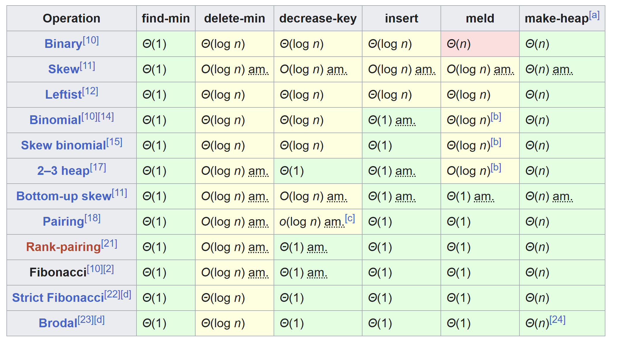
As we can see, the Fibonacci heap is theoretically the most efficient heap implementation, which is why algorithm textbooks invariably cover it. In practice, however, almost all mainstream implementations default to the binary heap, because binary heaps can be stored directly in an array without the overhead of maintaining numerous pointers as in a linked-list-based structure. Due to pointer operations, in real-world usage — especially when the data size is not enormous — a Fibonacci heap can actually be slower than the simplest binary heap.

It is worth noting the Pairing Heap, which performs very well in many practical settings and is one of the few heap implementations besides the binary heap that sees real-world use. Its structure is much simpler than a Fibonacci heap, and although its theoretical Decrease-Key complexity is \(O(\log \log n)\) (slightly worse than the Fibonacci heap's \(O(1)\)), it often outperforms the Fibonacci heap in actual benchmarks.

Let us briefly examine what a Fibonacci Heap is and how it differs from a binary heap.

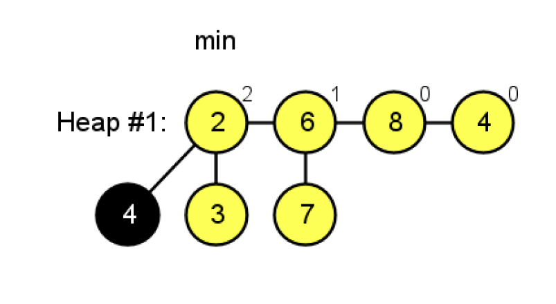
A binary heap is a single tree with strict ordering, whereas a Fibonacci heap is essentially a collection of trees (a forest). Each tree is not necessarily binary — each node can have any number of children. The roots of all trees are linked together via a doubly linked list (the root list), and we only need to maintain a pointer to the smallest root node at all times (the min pointer).

In a binary heap, every insertion or deletion triggers restructuring to ensure the heap remains a valid complete binary tree. A Fibonacci heap, by contrast, adopts a different strategy: restructuring only happens during EXTRACT-MIN — this is called the lazy strategy.

A Fibonacci heap does not need to be a complete binary tree, but it must still satisfy the heap property: the root node is less than or equal to (in a min heap) or greater than or equal to (in a max heap) its children. In other words, a Fibonacci heap may not be a complete binary tree and may consist of multiple trees:

1765220641206

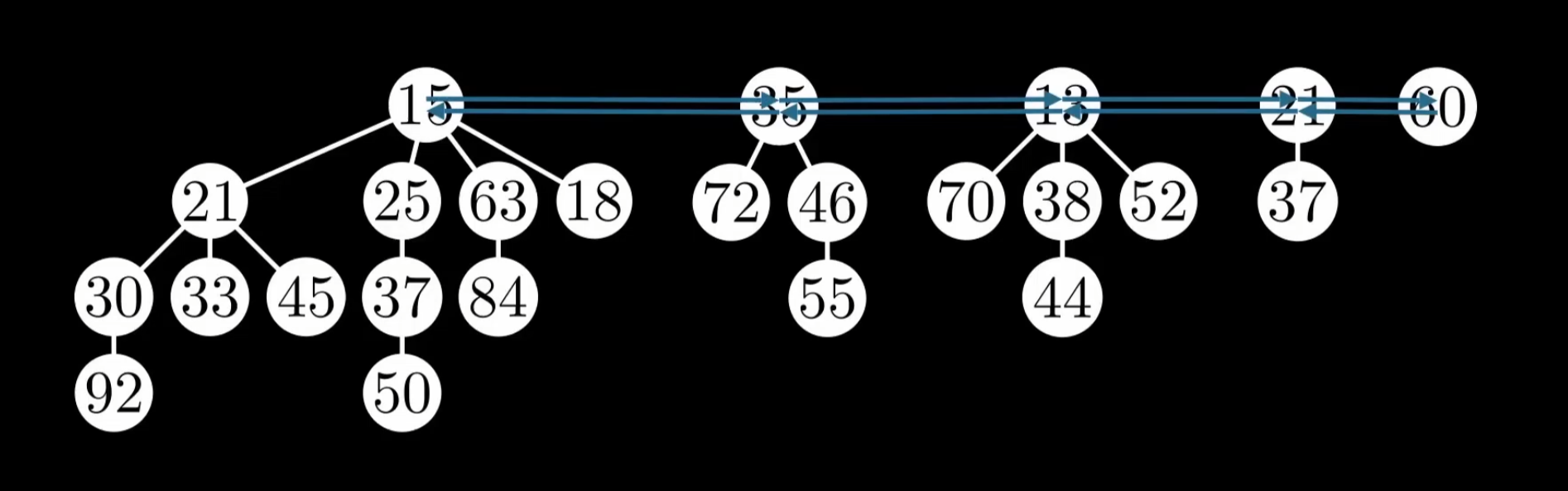
We store all tree roots in a doubly linked list — the root list. We track the position of the minimum node (the min pointer) to achieve O(1) FIND-MIN.

Moreover, within each tree at every level, the Fibonacci heap also uses a doubly linked list to connect all siblings, forming a sibling list.

With this design, the INSERT operation simply creates a new node and inserts it into the root list, typically right next to the min pointer. If the new node is smaller than the current minimum, the min pointer is updated to point to the new node. This makes INSERT O(1).

For the UNION operation, since two Fibonacci heaps H1 and H2 each have their own root list, we simply splice the two circular doubly linked lists together and then compare H1.min and H2.min, letting the smaller one become the new min pointer. The merge is complete in O(1).

In summary:

Insert: Simply toss the new node into the root list — O(1).
Union: Concatenate the two root lists and we are done — O(1).
Decrease-Key: When a node's value decreases, instead of sifting up, we directly cut the node from its parent, making it an independent tree in the root list. This operation is O(1) amortized.

These three optimizations are the hallmark strengths of the Fibonacci heap.

Decrease-Key

Let us elaborate on the Decrease-Key operation. First, recall the concept of degree: the degree of a node is the number of its direct children. If a root node is directly connected to 3 children, its degree is 3. Note that grandchildren, great-grandchildren, etc., do not count toward the degree — this is actually a concept from graph theory, and trees are special cases of graphs.

If we cut nodes arbitrarily, could we end up in a situation where all grandchildren have been cut away, but all direct children remain, causing the tree's node count to drop dramatically while the root's degree stays the same?

To prevent such deformities, cuts are performed using cascading cuts: as a non-root parent node, before you yourself get cut, you are only allowed to lose 1 child. When a child of root node's child A is cut, we immediately mark A as "marked." If another child of A is subsequently cut, then since A is already marked, A itself must be cut and moved to the root list.

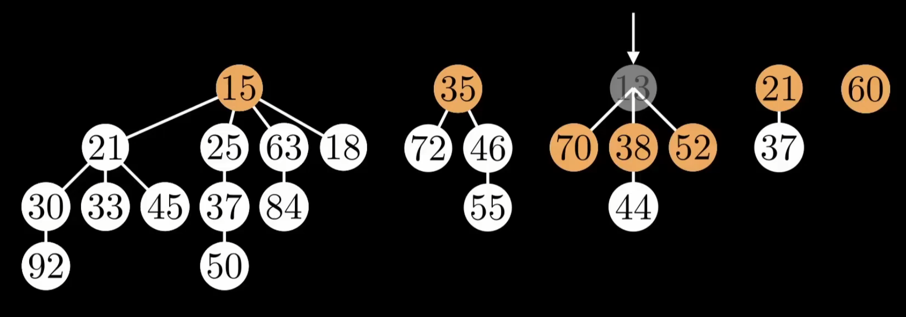
As shown in the figure below:

1765242311969

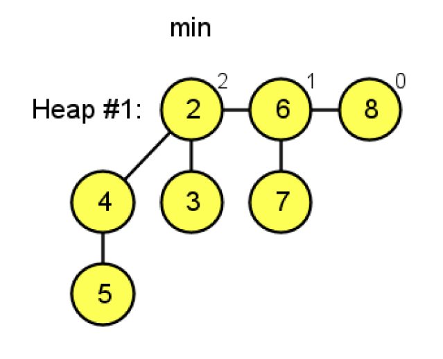
We perform a Decrease-Key operation on node 5. Because 5 is no longer greater than 4 (note: by standard theory, a cut is triggered only when the value becomes strictly less than the parent; however, the website used to generate this diagram also cuts on equality — under standard theoretical rules, equality does not require a cut), node 5 is cut. Then, according to cascading cut rules, the parent of the cut element is marked, as shown by the node being colored black:

1765242339055

Under cascading cut rules, a tree of degree k has a minimum number of nodes denoted \(N_k\). Suppose you are a node of degree \(k\). You have \(k\) children, arranged chronologically as \(y_1, y_2, ..., y_k\). According to the Fibonacci heap's linking rules, when the \(i\)-th child \(y_i\) was linked to you, you already had \(i-1\) children. So \(y_i\)'s degree at that time was at least \(\ge i-1\). The cascading cut rule stipulates: a child may lose at most 1 of its own children (otherwise it gets cut away and is no longer under you). Therefore, your \(i\)-th child \(y_i\) that is still under you now has a degree of at least \((i-1) - 1 = \mathbf{i-2}\).

To calculate the total node count \(N_k\), we sum the minimum number of nodes across all children, plus yourself (1 node). The degree sequence of the children (in the minimal case) is:

\(y_1\) (original degree 0 \(\to\) current degree 0): \(N_0\) nodes
\(y_2\) (original degree 1 \(\to\) current degree 0): \(N_0\) nodes
\(y_3\) (original degree 2 \(\to\) current degree 1): \(N_1\) nodes
\(y_4\) (original degree 3 \(\to\) current degree 2): \(N_2\) nodes
...
\(y_k\) (original degree \(k-1\) \(\to\) current degree \(k-2\)): \(N_{k-2}\) nodes

Formula:

\[ N_k = 1 + N_0 + N_0 + N_1 + N_2 + ... + N_{k-2} \]

Computing \(N_k\) from small values upward reveals the following recurrence:

\[ N_k = N_{k-1} + N_{k-2} \]

This is precisely the definition of the Fibonacci sequence. This is why this heap is named the Fibonacci heap.

Finally, let us examine the time complexity. Under the cascading cut rule, when a parent loses its first child, it gets marked — marking costs O(1) and we "store a coin." When a cascading cut occurs, the "coins" saved during marking pay for the cost. Therefore, no matter how long the cut chain is (the worst case being that each cut triggers another, leading to O(log N) cost), the expense is covered by the savings from earlier markings, thereby achieving O(1) amortized time complexity for Decrease-Key.

Extract-Min

Now let us look at Extract-Min. When performing EXTRACT-MIN, we need to find the new minimum from among the root list and the children of the deleted node:

1765220883161

However, due to prior INSERT and UNION operations — which create new root nodes upon insertion — the forest may have grown excessively large. For example:

1765221617423

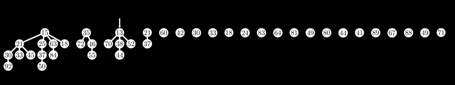
In this case, finding the next minimum after EXTRACT-MIN would be slow. If all N nodes had no children, finding the next minimum would degrade to O(N). To improve efficiency, the Fibonacci heap simultaneously performs two tasks:

Consolidation: merge trees with few or no children into new trees
Selection: find the new minimum (or maximum)

We consolidate the N candidate nodes on the field. This process is somewhat like a matching game: whenever two trees have the same degree, they must be merged. The core formula is: \(k + k \rightarrow k+1\):

Degree 0 + Degree 0 \(\rightarrow\) merged into a tree of Degree 1.
Degree 1 + Degree 1 \(\rightarrow\) merged into a tree of Degree 2.
Degree 2 + Degree 2 \(\rightarrow\) merged into a tree of Degree 3.
...and so on.

To accomplish this, we use an auxiliary bucket array A:

A[0]: temporarily stores the tree of degree 0.
A[1]: temporarily stores the tree of degree 1.
A[2]: temporarily stores the tree of degree 2.
...

Note that a bucket array of size 64 is typically sufficient to handle astronomically large datasets. If we never perform Decrease-Key, then the Fibonacci heap degenerates into a Binomial Heap, where a tree of degree \(k\) contains exactly \(2^k\) nodes. With \(N\) nodes, the maximum degree is \(D_{max} = \log_2 N\). If cuts have been performed, a tree of degree \(k\) contains at least \(F_{k+2} \approx \phi^k\) nodes (where \(\phi = 1.618\) is the golden ratio).

Derivation:

\[ N \ge 1.618^{D_{max}} \]

Taking logarithms of both sides:

\[ D_{max} \le \log_{1.618} N \]

Therefore, whether the base is 2 (binomial trees) or 1.618 (Fibonacci trees), as long as the node count grows exponentially, the degree (height) is necessarily \(O(\log N)\). This is why, after consolidation, the number of remaining trees (i.e., the maximum bucket index) is only \(\log N\).

In summary, the Extract-Min operation does not merely find the next minimum — it also consolidates the entire forest. The sole stopping criterion for consolidation is: after we have traversed all nodes in the root list (including original roots and newly promoted children), the auxiliary array A (bucket) must have at most one tree per degree slot.

This process is very similar to the game 2048. Suppose there are 32 nodes of degree 0; the entire consolidation proceeds as follows:

First, merge two 0s into a 1.
Merge two more 0s into a 1; now there are two 1s, so merge them into a 2.
Merge two more 0s into a 1, merge two more 0s into a 1; now there are two 1s, merge into a 2; now there are two 2s, merge into a 4.
...and so on.

For N nodes, the worst case costs O(N). However, since each insertion only cost O(1), the consolidation cost can be amortized to 0 — all consolidation expenses are offset by the savings from earlier insertions. If you are unfamiliar with amortized analysis, think of it this way: it is precisely the INSERT operations that create a large number of degree-0 trees, causing the consolidation overhead. So the work done by EXTRACT-MIN depends on the number of preceding insertions.

Consequently, we only need to consider the cost of finding the next minimum after consolidation. Since the bucket size is log N, the search complexity is naturally O(log N). Therefore, the total time complexity is: 0 + O(log N) = O(log N).

Worked Examples

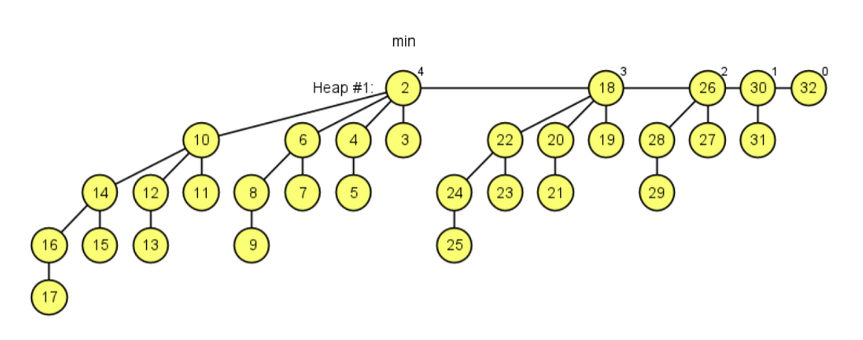
Example 1: Using Insert and Extract-Min operations, can you generate a Fibonacci heap whose root list contains five nodes with degrees 4, 3, 2, 1, and 0, respectively?

Solution:

Simply insert 32 numbers and then perform one Extract-Min to obtain the desired configuration. During the consolidation phase, the process resembles the game 2048:

1765239775699

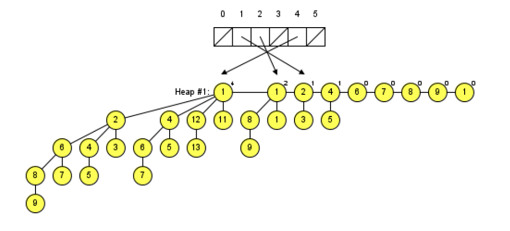
In a Fibonacci heap (after consolidation), the degree and tree size have a strict mathematical correspondence of \(2^k\):

A tree of degree 4 necessarily contains \(2^4 = \mathbf{16}\) nodes.
A tree of degree 3 necessarily contains \(2^3 = \mathbf{8}\) nodes.
A tree of degree 2 necessarily contains \(2^2 = \mathbf{4}\) nodes.
A tree of degree 1 necessarily contains \(2^1 = \mathbf{2}\) nodes.
A tree of degree 0 necessarily contains \(2^0 = \mathbf{1}\) node.

How many nodes are needed to have all these trees simultaneously in the heap? Sum the numbers above:

\[ 16 + 8 + 4 + 2 + 1 = \mathbf{31} \]

This means the heap must contain exactly 31 nodes after all operations are complete. To see the perfect consolidated form, the last operation must be Extract-Min. If the last operation were Insert, the newly inserted node would dangle as a degree-0 node alongside the others, breaking the desired perfect sequence (e.g., it would become 4, 3, 2, 1, 0, 0).

In other words, since 31 nodes must remain and the last operation must be Extract-Min, we must have 32 nodes before executing Extract-Min.

Example 2: We can see that in the generated result, the root node of the degree-4 tree has 4 children, whose degrees are 0, 1, 2, and 3, respectively. Explain why this property is preserved even after additional Extract-Min operations: a node of degree \(k\) has children with degrees \(0, 1, 2, \dots, k-1\) — exactly one child of each degree.

1765240607835

Answer:

After an Extract-Min operation, the Fibonacci heap performs consolidation by merging trees whose root nodes have the same degree, with the goal of eliminating duplicate degrees in the root list. This process is like the game 2048. When we merge two degree-0 root trees, we get one degree-1 root tree. When we merge two degree-1 root trees, we get one degree-2 root tree. This degree-2 root tree is formed by linking one degree-1 tree under the root of the other, so the degree-2 root has one degree-1 child (the tree that was just linked) plus its original child of degree 0. By induction, whenever we merge two trees of the same degree k, one tree of degree k is linked under the other's root. So when two degree-k root trees merge, the new degree-(k+1) tree gains a child subtree of degree k. Therefore, the stated property holds and is preserved regardless of how many Extract-Min operations are performed.

Example 3: Generate a Fibonacci heap containing trees of degrees 0, 1, 2, 3, 4, and 5, with each tree as full as possible. State the size of each tree. Then suppose all six trees undergo the maximum possible number of Decrease-Key operations without changing the degree of any tree's root. Explain how to obtain such a heap and state the size of each tree.

1765244026056

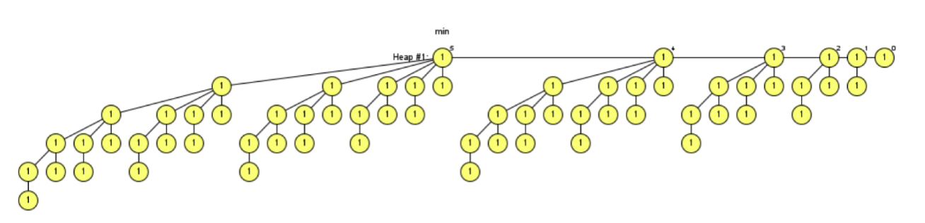
As before, we first insert 64 nodes and then perform one Extract-Min to obtain a full Fibonacci heap meeting the requirements.

The size of each tree is:

0-degree root tree: 1
1-degree root tree: 2
2-degree root tree: 4
3-degree root tree: 8
4-degree root tree: 16
5-degree root tree: 32

Next, we perform Decrease-Key operations. To maintain each root's degree while performing as many Decrease-Key operations as possible, the goal is to bring every child of every root into a marked state.

1765245435536

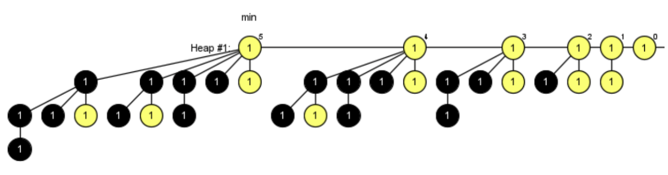
We omit the nodes that were cut and moved to the root list as a result of Decrease-Key operations.

As shown, the size of each tree is:

Degree 0: Size 1
Degree 1: Size 2
Degree 2: Size 3
Degree 3: Size 5
Degree 4: Size 8
Degree 5: Size 13

These are precisely the Fibonacci numbers. Through this example, we can intuitively see why the tree sizes after Decrease-Key operations follow the Fibonacci sequence.

Augmented Trees

The core idea of an augmented data structure is to store additional auxiliary information at each node of an existing data structure (such as a BST or red-black tree), thereby supporting more efficient query operations without changing the asymptotic complexity of the original operations.

The general methodology for augmentation (corresponding to CLRS Chapter 14) can be summarized in four steps:

Choose a base data structure (e.g., red-black tree)
Determine the additional information to maintain (e.g., subtree size size)
Verify that the additional information can be efficiently maintained during basic operations (insertions, deletions, and rotations can update it in \(O(\log n)\))
Develop new operations using the additional information (e.g., OS-SELECT, OS-RANK)

Order-Statistic Tree

The Order-Statistic Tree is a classic example of an augmented red-black tree. Each node \(x\) stores an additional attribute \(x.size\), representing the total number of nodes in the subtree rooted at \(x\) (including \(x\) itself).

           [26, size=7]
          /              \
    [17, size=3]      [41, size=3]
    /        \         /        \
[14, s=1] [21, s=1] [30, s=1] [47, s=1]

With the size attribute, the following two operations are supported:

Operation	Function	Time Complexity
OS-SELECT(x, i)	Find the \(i\)-th smallest element in the subtree rooted at \(x\)	\(O(\log n)\)
OS-RANK(T, x)	Return the rank of node \(x\) in the entire tree (its position in inorder traversal)	\(O(\log n)\)

Detailed pseudocode for OS-SELECT was provided in the OS-SELECT section under Red-Black Trees above. The idea behind OS-RANK is to walk from node \(x\) up to the root, accumulating the count of nodes to the left along the path.

The key to maintaining the size attribute is: during insertions and deletions, update the size of \(O(\log n)\) nodes along the path; during rotations, only the two nodes involved in the rotation need their size recomputed, at a cost of \(O(1)\). Therefore, the augmentation does not change the asymptotic complexity of the red-black tree.

Interval Tree

The Interval Tree is another example of an augmented red-black tree. Each node stores an interval \([low, high]\) and additionally maintains \(max\), the maximum right endpoint among all intervals in the subtree rooted at that node. With the \(max\) attribute, finding an interval that overlaps with a given query interval can be done in \(O(\log n)\) time.

B-Tree

A B-Tree is a self-balancing multi-way search tree designed for disk storage and database systems. Unlike binary trees, each node of a B-Tree can contain multiple keys and multiple children, thereby greatly reducing the tree's height and minimizing disk I/O operations.

Definition and Properties

A B-Tree with minimum degree \(t\) (\(t \ge 2\)) satisfies the following properties:

All leaf nodes are at the same level (perfectly balanced)
Each node contains at most \(2t - 1\) keys
Every non-root internal node contains at least \(t - 1\) keys
The root contains at least 1 key (unless the tree is empty)
An internal node with \(k\) keys has exactly \(k + 1\) children
Keys within a node are sorted in ascending order and satisfy the search tree property: all keys in child \(c_i\) \(<\) \(key_i\) \(<\) all keys in child \(c_{i+1}\)

Using a B-Tree with \(t = 2\) (also known as a 2-3-4 tree) as an example:

                    [16]
                   /    \
           [4, 8]        [20, 24]
          / |   \       /   |    \
       [1,2] [5,6] [9,10] [17,18] [21,22] [25,26]

Why It Is Suited for Disk Storage

The minimum unit of disk read/write is a disk page, typically 4KB. A B-Tree sets \(t\) to a large value (e.g., \(t = 1000\)) so that each node fills exactly one disk page. This way:

The tree height is \(O(\log_t n)\), far less than the \(O(\log_2 n)\) of a binary tree
With \(n = 10^9\) keys and \(t = 1000\), the tree height is only 3, meaning at most 3 disk I/O operations are needed to find a key

Core Operations

Search: Starting from the root, use linear search (or binary search) within the current node's key array to find the appropriate position. If a match is found, return it; otherwise, recurse into the corresponding child node. Each level accesses one node, so the number of disk I/O operations is \(O(h)\).

Insert: B-Tree insertion proceeds top-down. If a full node (containing \(2t-1\) keys) is encountered along the way, it is first split: the full node is divided into two halves, and the middle key is promoted to the parent. This ensures the target leaf node always has room for insertion.

Delete: Deletion is more complex and must handle three cases: deleting from a leaf, deleting from an internal node (replacing with predecessor or successor), and merging or borrowing when a node has too few keys.

Complexity

Operation	Time Complexity	Disk I/O
Search	\(O(t \log_t n)\)	\(O(\log_t n)\)
Insert	\(O(t \log_t n)\)	\(O(\log_t n)\)
Delete	\(O(t \log_t n)\)	\(O(\log_t n)\)
Space	\(O(n)\)	-

Here \(t\) is the cost of linear search within each node (or \(\log t\) if binary search is used), and \(\log_t n\) is the tree height. In practical database systems, \(t\) is a constant, so the time complexity of operations can be treated as \(O(\log n)\).

The B-Tree variant B+ Tree is more common in databases: all data is stored only in leaf nodes, internal nodes store only index keys, and leaf nodes are linked together via a linked list for efficient range queries.

Segment Tree

A Segment Tree is a tree-based data structure designed for handling range query and point update problems. It can perform range sum queries, range minimum/maximum queries, and other operations in \(O(\log n)\) time, while also supporting efficient element modifications.

Basic Idea

Given an array of length \(n\), a segment tree is a complete binary tree (usually stored in an array) where:

Each leaf node stores one element from the original array
Each internal node stores the aggregate result of its corresponding interval (e.g., interval sum, interval minimum, etc.)

Using the array [2, 1, 5, 3, 4] as an example, here is a range-sum segment tree:

                  [15]              -> sum of interval [0,4]
                /      \
            [8]          [7]        -> [0,2] and [3,4]
           /   \        /   \
        [3]    [5]    [3]    [4]    -> [0,1] [2,2] [3,3] [4,4]
       /   \
     [2]   [1]                      -> [0,0] [1,1]

Python Implementation

class SegmentTree:
    def __init__(self, data):
        self.n = len(data)
        self.tree = [0] * (4 * self.n)  # 开4倍空间
        self._build(data, 1, 0, self.n - 1)

    def _build(self, data, node, start, end):
        """建树：O(n)"""
        if start == end:
            self.tree[node] = data[start]
            return
        mid = (start + end) // 2
        self._build(data, 2 * node, start, mid)
        self._build(data, 2 * node + 1, mid + 1, end)
        self.tree[node] = self.tree[2 * node] + self.tree[2 * node + 1]

    def update(self, idx, val, node=1, start=0, end=None):
        """单点更新：将 data[idx] 修改为 val，O(log n)"""
        if end is None:
            end = self.n - 1
        if start == end:
            self.tree[node] = val
            return
        mid = (start + end) // 2
        if idx <= mid:
            self.update(idx, val, 2 * node, start, mid)
        else:
            self.update(idx, val, 2 * node + 1, mid + 1, end)
        self.tree[node] = self.tree[2 * node] + self.tree[2 * node + 1]

    def query(self, l, r, node=1, start=0, end=None):
        """区间查询：返回 [l, r] 的区间和，O(log n)"""
        if end is None:
            end = self.n - 1
        if r < start or end < l:
            return 0  # 完全不相交
        if l <= start and end <= r:
            return self.tree[node]  # 完全包含
        mid = (start + end) // 2
        left_sum = self.query(l, r, 2 * node, start, mid)
        right_sum = self.query(l, r, 2 * node + 1, mid + 1, end)
        return left_sum + right_sum


# 使用示例
data = [2, 1, 5, 3, 4]
seg = SegmentTree(data)
print(seg.query(1, 3))   # 输出 9 (1 + 5 + 3)
seg.update(2, 10)         # 将 data[2] 从 5 改为 10
print(seg.query(1, 3))   # 输出 14 (1 + 10 + 3)

Complexity

Operation	Time Complexity
Build	\(O(n)\)
Point Update	\(O(\log n)\)
Range Query	\(O(\log n)\)
Space	\(O(n)\) (array allocated as \(4n\))

Lazy Propagation

When range updates are needed (e.g., adding a value to all elements in \([l, r]\)), the naive approach requires updating \(O(n)\) leaf nodes individually. Lazy Propagation solves this by deferring updates: for intervals that are fully covered, a "pending update" tag is placed on the node, and the tag is only pushed down to children when a subsequent query or update needs to access those children. This reduces the complexity of range updates to \(O(\log n)\).

Van Emde Boas Tree

The Van Emde Boas Tree (vEB tree) is a data structure that supports efficient operations over an integer domain. When the universe of elements is \(\{0, 1, \dots, u-1\}\), a vEB tree can perform predecessor, successor, insert, and delete operations in \(O(\log \log u)\) time.

Core Idea

The key to the vEB tree is recursive blocking. The universe \(\{0, \dots, u-1\}\) is divided into \(\sqrt{u}\) blocks (clusters), each of size \(\sqrt{u}\), and a summary structure of size \(\sqrt{u}\) is maintained to record which clusters are non-empty. The summary itself is also a vEB tree.

For an element \(x\):

It belongs to cluster \(\lfloor x / \sqrt{u} \rfloor\) (called high(x))
Its position within the cluster is \(x \mod \sqrt{u}\) (called low(x))

The recursion depth is \(\log \log u\): \(u \to \sqrt{u} \to u^{1/4} \to u^{1/8} \to \cdots \to 2\). Each level does only \(O(1)\) work, so the total time is \(O(\log \log u)\).

Operations and Complexity

Operation	Time Complexity
Insert	\(O(\log \log u)\)
Delete	\(O(\log \log u)\)
Successor / Predecessor	\(O(\log \log u)\)
Find-Min / Find-Max	\(O(1)\)
Space	\(O(u)\)

Use Cases

The advantage of a vEB tree is that when \(u\) is not too large and frequent predecessor/successor queries are needed, \(O(\log \log u)\) is significantly better than the \(O(\log n)\) of a balanced BST. However, its space consumption is \(O(u)\), which is impractical when the universe is very large. In practice, hash tables can replace arrays for storing clusters (resulting in x-fast tries or y-fast tries) to mitigate the space issue.

Comparison with other structures:

Balanced BST (e.g., red-black tree): \(O(\log n)\), suitable for general scenarios, \(O(n)\) space
vEB tree: \(O(\log \log u)\), suitable for integer domains with manageable \(u\), \(O(u)\) space
Hash table: \(O(1)\) lookup, but does not support predecessor/successor

Fenwick Tree

A Fenwick Tree, also known as a Binary Indexed Tree (BIT), is a data structure that uses bit manipulation to efficiently handle prefix sum queries and point updates. Its functionality overlaps with that of a segment tree, but it is simpler to implement and has smaller constants.

Core Idea: lowbit

The essence of a Fenwick Tree lies in the lowbit operation, which extracts the lowest set bit in the binary representation of a positive integer:

\[ \text{lowbit}(x) = x \ \& \ (-x) \]

For example: \(\text{lowbit}(6) = \text{lowbit}(110_2) = 010_2 = 2\).

A Fenwick Tree uses an array tree[1..n] where tree[i] stores the sum of the original array from index \(i - \text{lowbit}(i) + 1\) to \(i\). The range managed by each position has length exactly lowbit(i).

Index i (binary)   lowbit(i)   Managed Range
  1   (0001)         1        [1, 1]
  2   (0010)         2        [1, 2]
  3   (0011)         1        [3, 3]
  4   (0100)         4        [1, 4]
  5   (0101)         1        [5, 5]
  6   (0110)         2        [5, 6]
  7   (0111)         1        [7, 7]
  8   (1000)         8        [1, 8]

Prefix sum query query(i): Starting from position \(i\), repeatedly subtract \(\text{lowbit}(i)\) and accumulate tree[i] along the way until \(i = 0\). Each jump clears the lowest set bit, so there are at most \(O(\log n)\) jumps.
Point update update(i, delta): Starting from position \(i\), repeatedly add \(\text{lowbit}(i)\) and update tree[i] along the way until \(i > n\). Similarly, there are at most \(O(\log n)\) jumps.

Python Implementation

class FenwickTree:
    def __init__(self, n):
        self.n = n
        self.tree = [0] * (n + 1)  # 下标从1开始

    def update(self, i, delta):
        """单点更新：将位置 i 的值加上 delta，O(log n)"""
        while i <= self.n:
            self.tree[i] += delta
            i += i & (-i)  # i += lowbit(i)

    def query(self, i):
        """前缀和查询：返回 [1, i] 的前缀和，O(log n)"""
        s = 0
        while i > 0:
            s += self.tree[i]
            i -= i & (-i)  # i -= lowbit(i)
        return s

    def range_query(self, l, r):
        """区间查询：返回 [l, r] 的区间和"""
        return self.query(r) - self.query(l - 1)

    @classmethod
    def from_array(cls, arr):
        """从数组建树，O(n)"""
        n = len(arr)
        bit = cls(n)
        bit.tree[1:] = arr[:]
        for i in range(1, n + 1):
            j = i + (i & (-i))
            if j <= n:
                bit.tree[j] += bit.tree[i]
        return bit


# 使用示例
data = [2, 1, 5, 3, 4]
bit = FenwickTree.from_array(data)
print(bit.range_query(2, 4))  # 输出 9 (1 + 5 + 3)
bit.update(3, 5)               # 将位置3的值加5（5 -> 10）
print(bit.range_query(2, 4))  # 输出 14 (1 + 10 + 3)

Complexity

Operation	Time Complexity
Build	\(O(n)\)
Point Update	\(O(\log n)\)
Prefix Sum Query	\(O(\log n)\)
Range Query	\(O(\log n)\)
Space	\(O(n)\)

Fenwick Tree vs Segment Tree

Comparison	Fenwick Tree	Segment Tree
Implementation complexity	Very concise (~20 lines)	More complex (requires recursive or iterative construction)
Constant factor	Small, faster in practice	Larger
Space	\(O(n)\)	\(O(4n)\)
Supported operations	Prefix sum query + point update	Arbitrary range queries + range updates (with Lazy Propagation)
Range update	Requires difference array tricks, limited extensibility	Natively supported (Lazy Propagation)
Use cases	Prefix sums, inversion counting, frequency statistics after discretization	Range min/max, range modifications, and other complex range operations

In short: if you only need prefix sums + point updates, prefer Fenwick Tree — the code is shorter and faster. If you need range updates or non-additive range queries (such as range min/max), use a Segment Tree.

Appendix: Classic Exercises

Binary Tree Basics

Diameter of a Tree

Maximum Depth

Minimum Depth

Balanced Binary Tree

Invert Binary Tree

Merge Binary Trees

Construct Binary Tree from Traversal Sequences

LCA (Lowest Common Ancestor)

Trie (Prefix Tree)

A Trie is a tree-based data structure designed specifically for string retrieval, where each edge represents a character.

Structure

class TrieNode:
    def __init__(self):
        self.children = {}  # char -> TrieNode
        self.is_end = False

class Trie:
    def __init__(self):
        self.root = TrieNode()

    def insert(self, word):
        node = self.root
        for c in word:
            if c not in node.children:
                node.children[c] = TrieNode()
            node = node.children[c]
        node.is_end = True

    def search(self, word):
        node = self.root
        for c in word:
            if c not in node.children:
                return False
            node = node.children[c]
        return node.is_end

Complexity

Insert/search: \(O(L)\), where \(L\) is the string length
Space: \(O(\Sigma \cdot N)\), where \(\Sigma\) is the alphabet size and \(N\) is the number of nodes

Applications

Autocomplete: Prefix search
Spell checking
IP routing: Longest prefix matching
Word frequency counting

Tree Structure Comparison

Data Structure	Search	Insert	Use Case
BST	\(O(\log n)\) avg	\(O(\log n)\) avg	Simple ordered data
AVL/Red-Black Tree	\(O(\log n)\)	\(O(\log n)\)	Strict balancing required
B-Tree	\(O(\log n)\)	\(O(\log n)\)	Disk storage/databases
Trie	\(O(L)\)	\(O(L)\)	String retrieval
Segment Tree	\(O(\log n)\)	\(O(\log n)\)	Range queries/updates
Fenwick Tree	\(O(\log n)\)	\(O(\log n)\)	Prefix sums/point updates
Heap	\(O(1)\) get extremum	\(O(\log n)\)	Priority queues

Tree

Tree Structures

Rooted Tree

Binary Tree

Traversal

Preorder Traversal

Inorder Traversal

Postorder Traversal

Complete Binary Tree

Full Binary Tree

BST

Predecessor and Successor

LCA (Lowest Common Ancestor)

BBST

AVL Tree

Rotations

Four Types of Imbalance

Red-Black Tree

OS-SELECT

Heap

Binary Heap

Core Operations

Fibonacci Heap

Worked Examples

Augmented Trees

Order-Statistic Tree

Interval Tree

B-Tree

Definition and Properties

Why It Is Suited for Disk Storage

Core Operations

Complexity

Segment Tree

Basic Idea

Python Implementation

Complexity

Lazy Propagation

Van Emde Boas Tree

Core Idea

Operations and Complexity

Use Cases

Fenwick Tree

Core Idea: lowbit

Python Implementation

Complexity

Fenwick Tree vs Segment Tree

Appendix: Classic Exercises

Binary Tree Basics

Diameter of a Tree

Maximum Depth

Minimum Depth

Balanced Binary Tree

Invert Binary Tree

Merge Binary Trees

Construct Binary Tree from Traversal Sequences

LCA (Lowest Common Ancestor)

Trie (Prefix Tree)

Structure

Complexity

Applications

Tree Structure Comparison

评论 #