Foundations of Deep Reinforcement Learning

These notes are primarily based on the lecture slides from UCB CS185/285 Deep Reinforcement Learning. https://rail.eecs.berkeley.edu/deeprlcourse/

Reinforcement Learning Review

Traditional supervised learning is given a dataset \(D = \{(x_i, y_i)\}\), and the model's objective is to learn a function \(f(x) \approx y\). Its core assumptions include:

• i.i.d. data: The data is assumed to be independently and identically distributed. This means that a photo of a cat you see today will not affect the photo of a dog the model sees tomorrow.
• Ground truth: During training, the model knows the correct \(y\) for each \(x\) (e.g., this image's label is "cat").

Reinforcement learning, on the other hand, operates more like a "closed-loop system":

• Non-i.i.d. data: This is RL's major pitfall. Previous outputs (actions) affect future inputs (states). For example, if a robot knocks over a stack of blocks, the scene it sees next changes completely.
• No ground truth: The system never tells you "move 5 centimeters to the left at this step." It only tells you at the end of the task (or along the way) whether you succeeded or failed (the reward mechanism).

The meaning of Independent and Identically Distributed (i.i.d.) includes two aspects:

1. Independence: Random variables do not influence each other. The data the model currently sees has no causal or logical connection to data it has seen before or will see in the future. For instance, when training a cat-vs-dog classifier, the first image is an orange tabby and the second is a husky. What these images are and the order they appear in have absolutely no effect on each other.
2. Identically Distributed: All data come from the same probability distribution (i.e., follow the same statistical patterns). The characteristics of the training data, the test data, and even data encountered in real-world deployment should all come from the same "pool." For example, if you train a face recognition model exclusively on Caucasian faces but deploy it in a scene with exclusively Asian faces, the identically distributed assumption is violated, and model performance will suffer significantly.

The core interaction framework of RL is the loop between the Agent and the Environment. At each time step \(t\), the agent observes state \(s_t\) and outputs action \(a_t\). The environment returns a reward \(r_t\) and the next state \(s_{t+1}\). The agent must "pick its own actions." The agent's ultimate goal is to learn a policy \(\pi_\theta : s_t \to a_t\) that maximizes the cumulative sum of rewards: \(\sum_t r_t\).

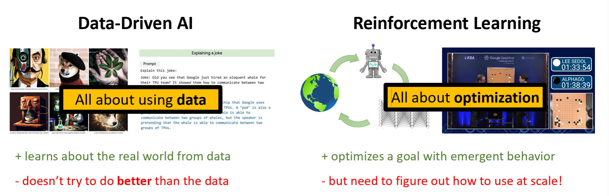
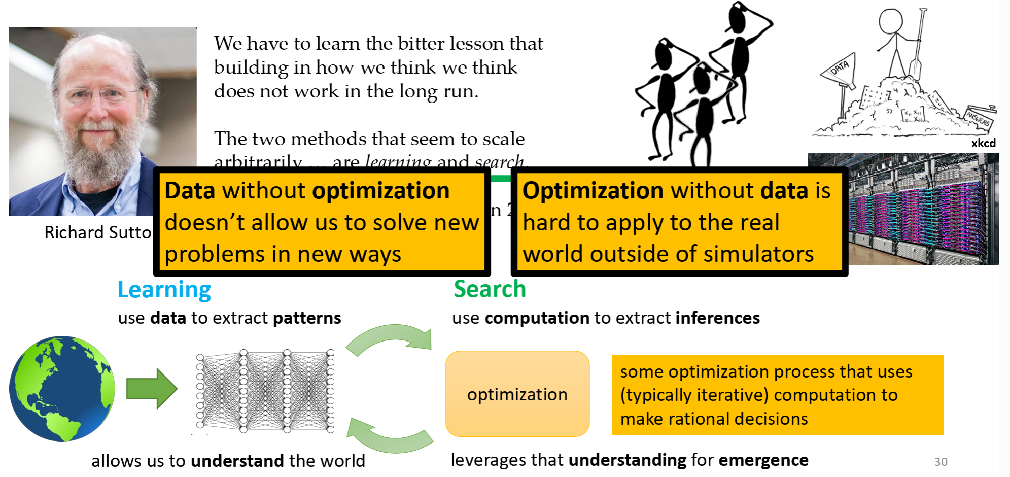
The value of RL lies in discovering novel solutions — it goes beyond merely imitating humans. AlphaGo's "divine move" fundamentally changed the game of Go, demonstrating that RL can discover solutions beyond human experience. Google Mind's absorption of Google Brain also reflects Google's emphasis on the reasoning-based approach.

Today, reinforcement learning is no longer a method exclusive to the robotics domain.

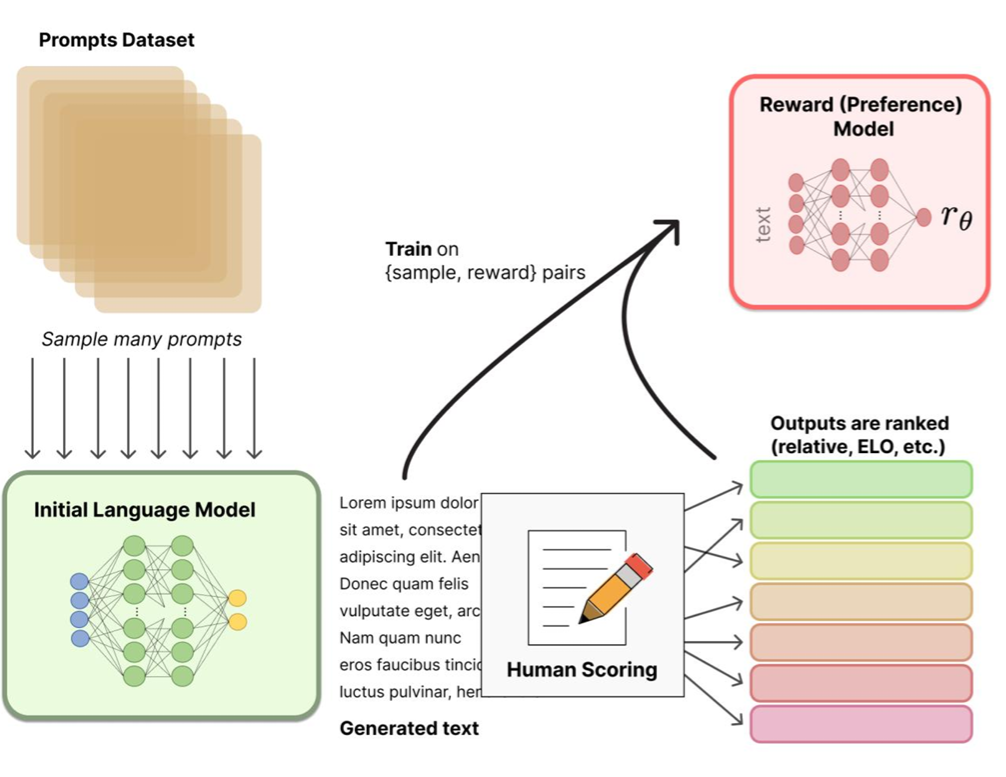
The figure above illustrates the core training mechanism behind modern large language models (such as ChatGPT): Reinforcement Learning from Human Feedback (RLHF):

1. Sampling and generation: Questions are sampled from a prompts dataset, and the initial model generates multiple different responses.
2. Human Scoring: Humans rank these responses (which is better, safer, more natural).
3. Reward Model: A "reward model" \(r_{\theta}\) is trained using the human ranking data. This model learns to approximate human preferences.
4. Model evolution: Finally, this reward model is used to guide updates to the original language model, making its outputs increasingly aligned with human expectations.

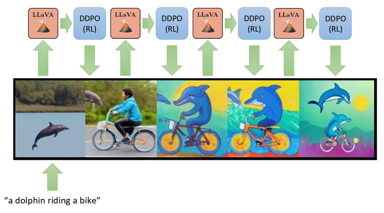
The figure above shows RL for image generation, where the key components include LLaVA and DDPO. LLaVA is a multimodal model that examines generated images and judges whether they match the text description (e.g., "a dolphin riding a bicycle"). DDPO refers to Denoising Diffusion Policy Optimization, which adjusts generation parameters based on LLaVA's feedback signal.

The evolution process can be understood as follows:

1. The initially generated image (leftmost) might just be an ordinary dolphin.
2. After multiple RL iterations, the model gradually learns the features of "riding a bicycle" and "anthropomorphism."
3. Eventually (rightmost), it produces an accurately composed, stylistically consistent "dolphin riding a bicycle" image.

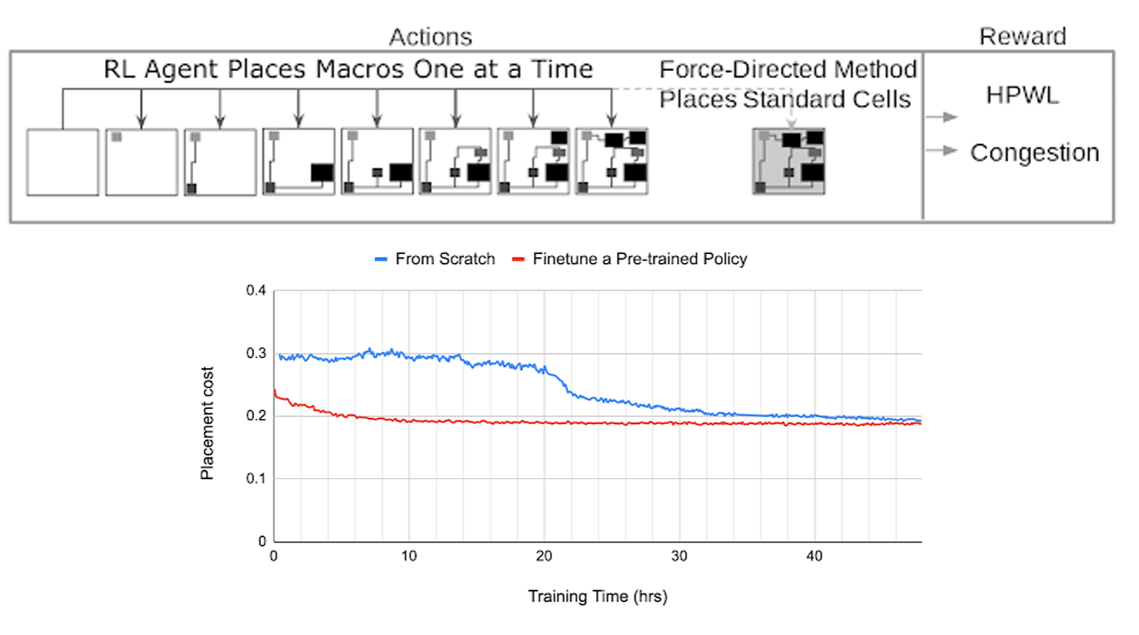
The figure above shows an application of RL in industrial automation: chip floorplan design. The task logic is based on actions and rewards:

• Actions: The RL agent places macro cells one after another, much like playing a jigsaw puzzle or Go.
• Reward: After placement, the system evaluates half-perimeter wire length (HPWL) and congestion. If the wiring is shorter and less congested, a higher score is given.

This demonstrates that RL can accomplish complex chip layout tasks in hours that would take human engineers weeks.

Behavioral Cloning

Behavioral Cloning (BC) is a machine learning technique that aims to train an agent by imitating human experts. It is the simplest and most direct form of Imitation Learning.

Behavioral cloning converts a control problem into a supervised learning problem:

1. The dataset consists of a series of "state-action" pairs \((s, a)\) demonstrated by an expert (e.g., a human driver). For instance, the expert sees a camera feed (state) and responds by turning the steering wheel (action).
2. The training objective is to learn a policy network \(\pi\) such that, given a state \(s\), the output action \(\pi(s)\) is as close as possible to the expert's action \(a\).

The most famous application of behavioral cloning dates back to the ALVINN system from the 1980s and the later NVIDIA self-driving experiments. ALVINN, developed by Dean Pomerleau at Carnegie Mellon University (CMU), is considered the pioneer of autonomous driving and behavioral cloning. At the time, it used an extremely simple neural network (with only one hidden layer) that learned by observing human drivers' steering behavior on the road.

It is worth noting that although the mathematical framework of reinforcement learning (such as Markov Decision Processes) matured during the 1950s–1980s, its powerful combination with deep learning (Deep RL) came much later. It was not until 2013–2016, with DeepMind's publication of the DQN paper on playing Atari games and the emergence of AlphaGo, that deep reinforcement learning truly entered the public spotlight.

Maximum Likelihood Estimation

Let us examine the formal definition of behavioral cloning.

Suppose we have a dataset \(\mathcal{D}\) of expert demonstrations containing \(N\) trajectories:

\[ \mathcal{D} = \{ (s_0, a_0), (s_1, a_1), \dots, (s_t, a_t) \} \]

where:

• \(s_t \in \mathcal{S}\): the state at time \(t\).
• \(a_t \in \mathcal{A}\): the action taken by the expert in state \(s_t\).

Now we adopt a function that takes s as input and produces a as output. We want this function to always behave as a human would — in other words, we can have the function learn from the dataset:

\[ f_{\theta}(s) \approx a_{human} \]

If we use a neural network, then we are essentially looking for a set of parameters \(\theta\) (the neural network's weights) that make the network's output consistently close to our dataset \(\mathcal{D}\). We call this neural network function the policy \(\pi_{\theta}(a|s)\).

Note that what we are discussing here is supervised learning, not reinforcement learning, since there is no agent trial-and-error involved. Therefore, we typically apply maximum likelihood estimation here — finding a set of parameters \(\theta\) that maximizes the probability of predicting the correct labels.

\[ \arg \max_\theta \sum_{i=1}^N \log p_\theta(y^{(i)}|\mathbf{x}^{(i)}) \]

---

However, for real-world problems, we clearly need to introduce sequential decision-making. We can introduce a time step \(t\) and define the following variables:

• \(\mathbf{s}_t\): State — the true physical state of the environment.
• \(\mathbf{o}_t\): Observation — the image or sensor data that the agent perceives.
• \(\mathbf{a}_t\): Action — the decision made by the agent (e.g., turning the steering wheel).
• \(\pi_\theta(\mathbf{a}_t | \mathbf{o}_t)\): Policy — the neural network model we need to learn.

Note that in policy learning for imitation learning, we typically do not need to know the environment's dynamics model (i.e., \(p(\mathbf{s}_{t+1}|\mathbf{s}_t, \mathbf{a}_t)\)) or the observation model (\(p(\mathbf{o}_t|\mathbf{s}_t)\)). We only focus on learning the policy \(\pi_\theta\). We should also be aware of two scenarios:

1. Partially Observed: The agent can only see observations \(\mathbf{o}_t\) (such as a camera feed), which are a subset or transformation of the true state \(\mathbf{s}_t\).
2. Fully Observed: We assume the observation equals the true state, i.e., \(\mathbf{o}_t = \mathbf{s}_t\).

The above constitutes the Sequential Decision Making process.

---

When we directly apply supervised learning to sequential decision-making tasks, we obtain the general method of Behavioral Cloning. In behavioral cloning, the data is no longer a simple \((x, y)\) pair, but rather expert demonstration trajectories:

• The dataset contains \(N\) trajectories, each consisting of \(H\) time steps.
• The data takes the form: \(\{(\mathbf{o}_t^{(i)}, \mathbf{a}_t^{(i)})\}\) — meaning "when seeing a particular image \(\mathbf{o}\), the expert took action \(\mathbf{a}\)."

The learning process is as follows:

• Input: The current observation \(\mathbf{o}_t\) (e.g., a dashcam image).
• Output: The predicted action \(\mathbf{a}_t\) (e.g., steering angle, throttle).
• Objective function: Nearly identical to standard supervised learning — the goal is to maximize the log-likelihood of expert actions under the policy distribution:

\[ \arg \max_\theta \sum_{i=1}^N \sum_{t=1}^H \log \pi_\theta(\mathbf{a}_t^{(i)}|\mathbf{o}_t^{(i)}) \]

Just like teaching a student to solve problems, the neural network (student) observes a large number of "see road conditions -> perform action" samples from human drivers (teacher) and simply mimics the teacher's responses in specific situations.

Loss Function

Above, we established the general guiding principle of behavioral cloning: using maximum likelihood estimation to maximize the probability of expert actions.

Now let us examine how to concretely implement this principle. We can choose an appropriate loss function based on the type of action space.

---

For discrete actions, we use softmax to convert scores into probabilities.

\[ p(a_t=k | o_t) = \frac{\exp(f_k(o_t))}{\sum_j \exp(f_j(o_t))} \]

The loss function typically uses cross-entropy loss.

---

For continuous actions, we usually output the parameters of a Gaussian distribution — the mean \(\mu(o_t)\) and covariance \(\Sigma(o_t)\).

\[ p(a_t | o_t) = \mathcal{N}(a_t | \mu(o_t), \Sigma(o_t)) \]

If we assume the variance \(\Sigma\) is a constant matrix \(\mathbf{I}\), then maximizing the log-likelihood is equivalent to minimizing the mean squared error (MSE):

\[ \text{Loss} \propto ||\mathbf{a}_t - \mu(\mathbf{o}_t)||^2 \]

That is, making the neural network's output "action mean" as close as possible to the "expert's actual action."

The principle here is that if we assume the error follows a Gaussian distribution, then maximizing probability is mathematically equivalent to minimizing the squared distance between the two values:

\[ \text{Maximize Probability} \iff \text{Minimize } ||\text{predicted} - \text{actual}||^2 \]

.

---

To summarize, the general formula for both cases above is \(\arg \max \log \pi\). In engineering practice, we choose the appropriate loss function based on the output type:

• For classification tasks, such as AlphaGo's move selection, we use cross-entropy loss.
• For regression tasks, such as autonomous driving steering angles, we use MSE loss.

Distribution Shift

The mathematical principles above demonstrate that naive behavioral cloning often causes the policy to produce trajectories that deviate from expert trajectories. Behavioral cloning cannot guarantee that it will always work. It has fundamental differences from traditional supervised learning.

The core reason for behavioral cloning's failure is distributional shift.

The central assumption of supervised learning is that training data and test data are independently and identically distributed (i.i.d.). That is, \(p_{train}(x) \approx p_{test}(x)\). However, this assumption does not hold in BC.

Let us examine the error accumulation process in BC:

1. We train the model under the expert's state distribution \(p_{data}(o_t)\).
2. During testing, the model inevitably produces small errors \(\epsilon\).
3. These small errors cause the agent to enter a new state that slightly deviates from the expert trajectory.
4. Because this new state has never appeared (or appeared with very low probability) in the training data, the model's behavior becomes unpredictable, leading to even larger errors.
5. Eventually, the state distribution \(p_{\pi_\theta}\) completely diverges from the training distribution \(p_{data}\), causing system failure (e.g., the car drives off the road).

If we define:

• \(H\): The trajectory length (horizon).
• \(\epsilon\): The probability that the model makes an error on the training distribution (i.e., \(\mathbb{E}_{s \sim p_{train}} [\pi_\theta(a \neq \pi^*(s))] \le \epsilon\)).
• Goal: Estimate the total number of errors during testing.

Through mathematical derivation, we can obtain the worst-case result, where the error upper bound is \(O(\epsilon H^2)\). We skip the detailed derivation here, but the key point for comparison is that traditional supervised learning error is typically linear at \(O(\epsilon H)\). As the horizon \(H\) increases, the quadratic error growth in behavioral cloning causes performance to deteriorate rapidly.

Although the theoretical worst-case bound of \(O(\epsilon H^2)\) is quite pessimistic, in practice (e.g., NVIDIA's cars), BC often works. This may be because the data contains segments where the driver "drifts off course and then corrects back to center" rather than being a perfect expert demonstration, so the model learns how to self-correct under distribution shift.

We can also use algorithms like DAgger (Dataset Aggregation). It continuously collects data from states where the agent has drifted off course, asks the expert to label the correct actions, and forcibly adds these "drifted states" to the training set, thereby correcting distribution shift.

To summarize, common solutions for distribution shift and error accumulation include:

1. Annotating erroneous actions in the dataset, or collecting and labeling data from drifted states.
2. Using more powerful models to drive \(\epsilon\) (training error) as low as possible. If \(\epsilon\) is very small, even \(H^2\) growth is acceptable.
3. Deliberately injecting noise (perturbations) into the data, forcing the model to learn how to recover from deviations.
4. Using multi-task learning to improve the model's generalization ability.

Imitation Learning

Above, we introduced behavioral cloning, which is the most basic and intuitive form of Imitation Learning (IL). The essence of behavioral cloning is supervised learning, while imitation learning is a broader category that shares the same fundamental goal: enabling agents to learn policies by observing expert demonstrations.

Beyond the basic behavioral cloning introduced above, imitation learning has evolved into various schools and directions today, including:

1. Temporal imitation learning — incorporating non-Markovian decisions by considering temporal dependencies, using architectures such as RNN and Transformer.
2. Interactive imitation learning — DAgger belongs to this category.
3. Inverse reinforcement learning.
4. Generative adversarial imitation learning.
5. Flow Matching.

MDP

Above, we discussed imitation learning and behavioral cloning, two methods that were very important in the early development of reinforcement learning. The core logic is like teaching a child to drive: we show the AI large amounts of human driving videos and operation records. The AI's goal is to learn a policy \(\pi_\theta(a_t | s_t)\) — that is, when seeing the current road conditions (state \(s_t\)), output actions as similar to the human's as possible (action \(a_t\), such as turning the steering wheel or pressing the accelerator):

\[ \arg \max_\theta \sum_{i=1}^N \sum_{t=1}^H \log \pi_\theta(a_t^{(i)} | s_t^{(i)}) \]

This is essentially a supervised learning problem. By maximizing the likelihood function, we make the model parameters \(\theta\) predict the actions that the expert would take in specific states. However, what if we do not have good demonstration data? What if the AI makes a small mistake and drifts away from the expert's trajectory? This motivates the need for reinforcement learning.

Markov Chain

Before diving into the complexities of reinforcement learning, we must understand the simplest probabilistic model — the Markov Chain.

Let us define a system that does not consider "actions" and only considers "state evolution." This system obeys the Markov Property:

\[ s_{t+1} \perp s_{t-1} | s_t \]

The core idea is: the future depends only on the present, not on the past. Once the current state \(s_t\) is known, the past trajectory provides no additional help in predicting \(s_{t+1}\).

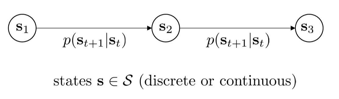
We use \(p(s_{t+1} | s_t)\) to denote the probability of transitioning from one state to the next. If you write the probability distribution over all states as a vector \(\mu_t\), then the distribution at the next time step can be obtained through matrix multiplication: \(\mu_{t+1} = \mathcal{T} \mu_t\).

MDP

When we add actions and rewards to a Markov Chain, it becomes an MDP (Markov Decision Process). This is the standard formulation of reinforcement learning.

Its core components include:

1. State \(s_t\)****: The road conditions.
2. Action \(a_t\)****: Accelerating or steering.
3. Reward function \(r(s_t, a_t)\)****: This is the most critical addition. Instead of blindly imitating humans, the system judges quality through "reward signals."
   • High reward: Safe and smooth driving (the sports car in the figure).
   • Low/negative reward: A collision (the car crash in the figure).
4. Transition probability \(p(s_{t+1} | s_t, a_t)\)*: The probability that the environment transitions to *\(s_{t+1}\) given state \(s_t\) and action \(a_t\).

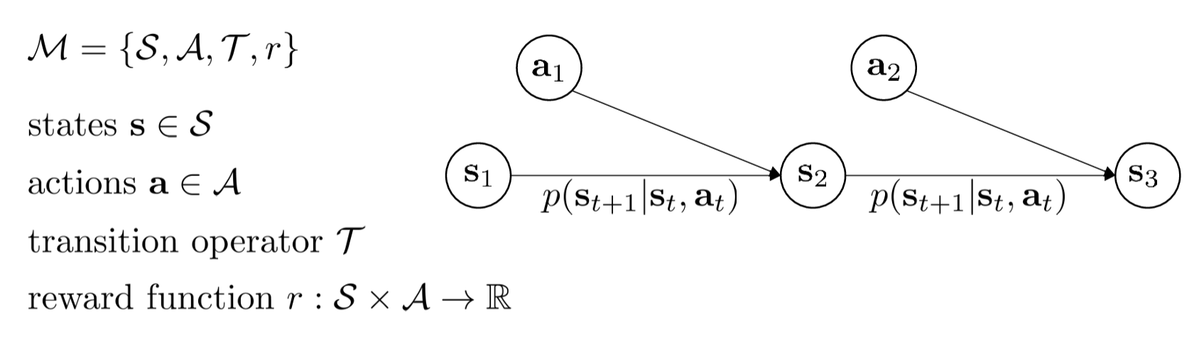
As shown in the figure above, this is a very standard MDP:

1. \(\mathcal{S}\) (States): The state space — all possible situations the environment can be in.
2. \(\mathcal{A}\) (Actions): The action space — all operations the agent can take.
3. \(\mathcal{T}\) (Transition Operator): The transition operator, i.e., \(p(\mathbf{s}_{t+1} | \mathbf{s}_t, \mathbf{a}_t)\). It describes the probability of the environment entering the next state after a certain action is taken in the current state.
4. \(r\) (Reward Function): The reward function \(r: \mathcal{S} \times \mathcal{A} \to \mathbb{R}\). It tells the agent how many immediate points it receives for taking action \(\mathbf{a}\) in state \(\mathbf{s}\).

The mathematical properties of Markov Chains (which have only state transitions and no actions) are elegant and easy to work with. So when we introduce "actions" and "policies," can we still leverage those elegant mathematical tools? The answer is yes — we can fix the policy pi and treat the state-action pair (s, a) as a new augmented state. Then:

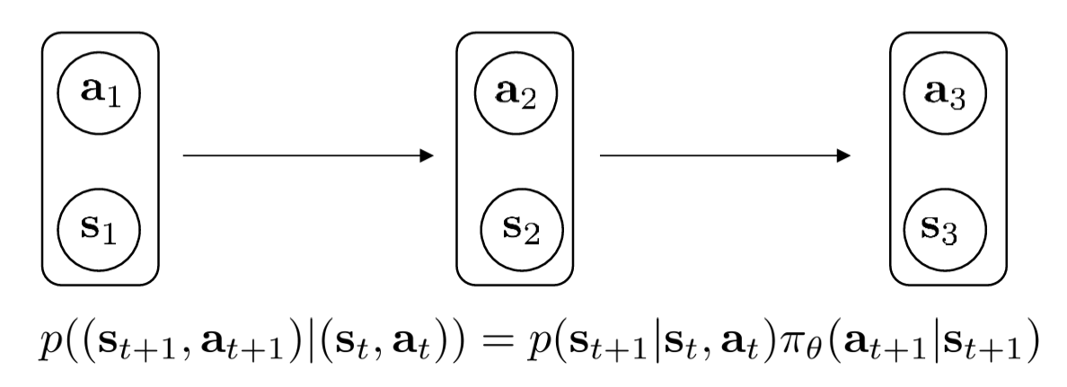
The formula above:

\[ p((\mathbf{s}_{t+1}, \mathbf{a}_{t+1}) | (\mathbf{s}_t, \mathbf{a}_t)) = p(\mathbf{s}_{t+1} | \mathbf{s}_t, \mathbf{a}_t) \pi_\theta(\mathbf{a}_{t+1} | \mathbf{s}_{t+1}) \]

can be decomposed into two steps:

1. The environment's step: \(p(\mathbf{s}_{t+1} | \mathbf{s}_t, \mathbf{a}_t)\) — given the current state and action, the environment determines the next state.
2. The agent's step: \(\pi_\theta(\mathbf{a}_{t+1} | \mathbf{s}_{t+1})\) — after observing the new state, the policy \(\pi\) determines the next action.

This construction offers two major mathematical advantages:

• Model simplification: Once you fix a policy \(\pi\), the entire MDP collapses into a Markov Chain.
• Long-term behavior analysis: We can leverage Markov Chain properties (such as stationary distributions) to analyze which states the robot will frequent if it follows this policy for a long time. This is crucial for computing "expected returns."

POMDP

In the MDP described above, the agent can directly observe the state \(s_t\). However, in real-world problems, we typically do not have a god's-eye view — we can only guess the state through observations. This leads us to the Partially Observed Markov Decision Process (POMDP).

Two new elements are introduced:

• New variable \(\mathcal{O}\) (Observations): The sensor data the agent actually receives (e.g., camera images, radar signals).
• New operator \(\mathcal{E}\) (Emission Operator): Expressed probabilistically as \(p(\mathbf{o}_t | \mathbf{s}_t)\). It describes the probability of producing a particular observation given the current true state.

For example, the true state \(\mathbf{s}_t\) is that there is a car behind you, but your rearview mirror has a blind spot, so your observation \(\mathbf{o}_t\) does not include it.

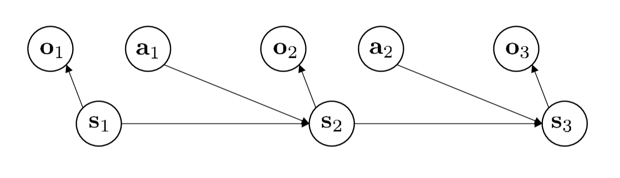
As shown in the figure above, we can see the connections in the diagram:

1. \(\mathbf{s}_1 \to \mathbf{o}_1\): The true state determines what you observe.
2. \(\mathbf{s}_1, \mathbf{a}_1 \to \mathbf{s}_2\): The physical world evolves based on the current state and your action, producing the next true state \(\mathbf{s}_2\).
3. \(\mathbf{s}_2 \to \mathbf{o}_2\): And so on — you receive a new observation.

The key point here is: Action \(\mathbf{a}_t\) is now based on observation \(\mathbf{o}_t\) (or the history of all past observations), not on the hidden state \(\mathbf{s}_t\).

POMDPs are quite complex (they are PSPACE-complete problems). For now, let us assume that the sensors (cameras, LiDAR, etc.) are sufficiently comprehensive to represent the current state — that is, we assume full observability.

Trajectory Distribution

The figure below shows the interaction loop between the Agent and the Environment (Earth), along with the joint probability formula for trajectories: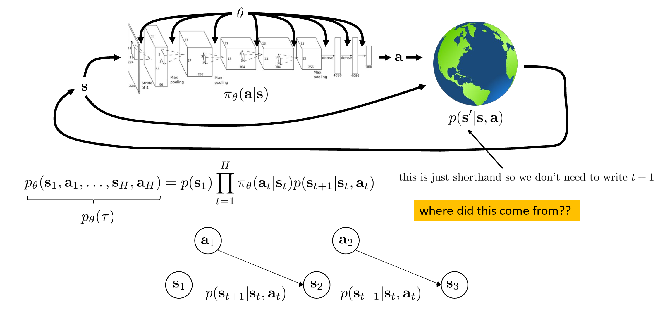

A trajectory \(\tau\) refers to a complete sequence: state, action, state, action... \(\tau = (\mathbf{s}_1, \mathbf{a}_1, \dots, \mathbf{s}_H, \mathbf{a}_H)\).

The interaction loop:

• Policy \(\pi_\theta(\mathbf{a}|\mathbf{s})\)*: Represented by a neural network — it takes the current state *\(\mathbf{s}\) as input and outputs an action \(\mathbf{a}\).
• Environment \(p(\mathbf{s}'|\mathbf{s}, \mathbf{a})\)*: The earth icon represents the environment, which determines the next state *\(\mathbf{s}'\) based on the current state and your action (here \(\mathbf{s}'\) is shorthand for \(\mathbf{s}_{t+1}\)).

This yields the trajectory distribution \(p_\theta(\tau)\)**:

\[ p_\theta(\mathbf{s}_1, \mathbf{a}_1, \dots, \mathbf{s}_H, \mathbf{a}_H) = p(\mathbf{s}_1) \prod_{t=1}^H \pi_\theta(\mathbf{a}_t|\mathbf{s}_t) p(\mathbf{s}_{t+1}|\mathbf{s}_t, \mathbf{a}_t) \]

This formula is essentially the chain rule of probability theory:

1. \(p(\mathbf{s}_1)\): Where you are born (initial state probability).
2. \(\pi_\theta(\mathbf{a}_t|\mathbf{s}_t)\): At each time step, the action you choose according to your policy.
3. \(p(\mathbf{s}_{t+1}|\mathbf{s}_t, \mathbf{a}_t)\): How the environment pushes you to the next state based on your action.

The yellow question in the figure ("where did this come from") arises from the Markov property. Because the future depends only on the current state and action, we can write the probability of the entire sequence as the product of these terms.

This formula and concept are very practical — it is worth keeping in mind.

State Marginal Distribution

What if we do not care about the entire "life trajectory" but only care about "at time \(t\), what is the probability of being in state \(\mathbf{s}_t\)?" In other words, if you follow a certain policy \(\pi_\theta\), at a specific time point \(t\), what is the probability of being at a particular position \(\mathbf{s}_t\)?

\[ p_\theta(\mathbf{s}_t) = \sum_{\mathbf{a}_{1:H}, \mathbf{s}_{1:t-1}, \mathbf{s}_{t+1:H}} p_\theta(\mathbf{s}_1, \mathbf{a}_1, \dots, \mathbf{s}_H, \mathbf{a}_H) \]

\[ = \sum_{\mathbf{a}_{1:t-1}, \mathbf{s}_{1:t-1}} p(\mathbf{s}_1) \prod_{t'=1}^{t-1} \pi_\theta(\mathbf{a}_{t'}|\mathbf{s}_{t'}) p(\mathbf{s}_{t'+1}|\mathbf{s}_{t'}, \mathbf{a}_{t'}) \]

What if we just want to sample from this marginal distribution? If you try to compute it using the complex summation formula above, the computational cost is astronomical — utterly infeasible. But in practice (or in code), it is trivially simple:

1. Let your AI take the current policy \(\pi_\theta\) and actually run it in the environment.
2. At time step \(t\), stop and record the current state \(\mathbf{s}_t\).
3. This recorded \(\mathbf{s}_t\) is a sample drawn from the marginal distribution.

If you run 1000 times, the distribution of these 1000 positions is the shape represented by that complex mathematical formula.

This formula and concept are very practical — it is worth keeping in mind.

Objective Function

Trajectory Perspective

The standard objective function of RL is:

\[ \theta^\star = \arg \max_\theta \mathbb{E}_{\tau \sim p_\theta(\tau)} \left[ \sum_t r(\mathbf{s}_t, \mathbf{a}_t) \right] \]

That is, we want to find a set of optimal parameters \(\theta^\star\) (typically neural network weights) that maximize the expected value of the cumulative reward sum over the entire trajectory (\(\tau\)).

\(r(\mathbf{s}_t, \mathbf{a}_t)\) represents the reward obtained by taking action \(\mathbf{a}_t\) in state \(\mathbf{s}_t\). It tells the agent which states and actions are desirable. We must optimize long-term reward. For example, if we are training a policy for self-driving cars and only look at immediate rewards, the agent will fail to avoid future chain reactions (such as car crashes).

To compute the expectation above, we need to understand how a "process" (trajectory) unfolds:

\[ p_\theta(\mathbf{s}_1, \mathbf{a}_1, \dots, \mathbf{s}_H, \mathbf{a}_H) = p(\mathbf{s}_1) \prod_{t=1}^H \pi_\theta(\mathbf{a}_t|\mathbf{s}_t) p(\mathbf{s}_{t+1}|\mathbf{s}_t, \mathbf{a}_t) \]

This formula describes the trajectory generation logic:

1. \(p(\mathbf{s}_1)\): The initial state.
2. \(\pi_\theta(\mathbf{a}_t|\mathbf{s}_t)\): The policy. The probability that the agent chooses action \(a\) in state \(s\) given parameters \(\theta\).
3. \(p(\mathbf{s}_{t+1}|\mathbf{s}_t, \mathbf{a}_t)\): The environment transition. How the environment changes to the next state after an action is taken.

Reinforcement learning is not just about learning the correct action at the present moment. By optimizing the policy parameters \(\theta\), it enables the agent to accumulate as much total reward as possible over an extended future time horizon, accounting for the uncertainty inherent in environmental interactions.

Marginal Distribution Perspective

Above, we discussed the trajectory-perspective objective function:

\[ J(\theta) = \mathbb{E}_{\tau \sim p_\theta(\tau)} \left[ \sum_{t=1}^H r(\mathbf{s}_t, \mathbf{a}_t) \right] \]

This is the most intuitive RL objective to understand. The agent walks through the environment from start to finish, forming a complete sequence of experiences — this is the trajectory (\(\tau\)). We want to find the best policy \(\theta\) such that, among all possible trajectories generated under this policy, the "expected total reward" is maximized. To compute this expectation, you need to know the probability of the entire trajectory \(\tau\) (the long chain of products from earlier). If we only run a few time steps \(H\), this is still feasible; but if the environment runs indefinitely (\(H \to \infty\)), this infinitely long product of probabilities becomes mathematically intractable — the formula simply "dies" here.

Instead of asking "what is the probability of this complete trajectory," we can ask "at time step \(t\), what is the probability of being exactly in state \(\mathbf{s}_t\) and taking action \(\mathbf{a}_t\)?" We compute the expected reward at each individual time step, then sum over all time steps.

\[ \sum_{t=1}^H \mathbb{E}_{\mathbf{s}_t, \mathbf{a}_t \sim p_\theta(\mathbf{s}_t, \mathbf{a}_t)} [r(\mathbf{s}_t, \mathbf{a}_t)] \]

We have avoided computing the product over the entire trajectory, but \(p_\theta(\mathbf{s}_t, \mathbf{a}_t)\) (the probability of being in a specific state-action pair at step \(t\)) is still quite complex when expanded, involving many summation terms. We need more concise mathematical tools to express it.

Matrix Perspective

To make the formulas cleaner and amenable to computer implementation and existing mathematical theorems, we introduce linear algebra. We enumerate all possible state-action combinations and arrange them into a long vector:

• Define \(p_\theta(\mathbf{s}_t, \mathbf{a}_t)\) as the column vector \(\mu_t\) (the probability distribution at step \(t\)).
• Define the reward corresponding to each state-action pair as the column vector \(\vec{r}\).
• Define the transition probability from one step to the next as a large transition matrix \(\mathcal{T}_\theta\).

Time-step progression becomes a simple matrix multiplication:

\[ \mu_{t+1} = \mathcal{T}_\theta \mu_t \]

And the originally complex total objective function becomes a sum of vector dot products:

\[ \sum_{t=1}^H \mu_t^T \vec{r} \]

In Markov Chain theory, if a transition matrix \(\mathcal{T}_\theta\) is repeatedly multiplied (as time progresses), the probability distribution vector \(\mu_t\) eventually stops changing and stabilizes at a fixed distribution. This final stable vector is called the stationary distribution (\(\bar{\mu}\)).

Since the distribution no longer changes, multiplying by the transition matrix yields itself:

\[ \bar{\mu} = \mathcal{T}_\theta \bar{\mu} \implies (\mathcal{T}_\theta - \mathbf{I})\bar{\mu} = 0 \]

At this point, the expected reward per step over an infinitely long horizon is elegantly condensed into the dot product of the stationary distribution vector and the reward vector:

\[ J(\theta) = \bar{\mu}^T \vec{r} \]

This final simplified form \(\bar{\mu}^T \vec{r}\) is the ultimate reduced form of the objective function for reinforcement learning under the infinite horizon setting. It represents: the expected reward per step that the agent can obtain over long-term operation.

Monte Carlo Estimation

Above, we discussed complex mathematical theory. In practice, we generally perform sampling, and the resulting trajectories are called rollouts. We randomly draw batches from rollouts to train the policy network.

In engineering practice, this approach can be written as:

\[ \mathbb{E}_{\tau \sim p_\theta(\tau)} \left[ \sum_{t=1}^H r(\mathbf{s}_t, \mathbf{a}_t) \right] \approx \frac{1}{N} \sum_{i=1}^N \left( \sum_{t=1}^H r(\mathbf{s}_t^{(i)}, \mathbf{a}_t^{(i)}) \right) \]

The left-hand side is the theoretical expectation. This is the absolute truth that the earlier slides painstakingly tried to compute using Markov Chains, transition matrices, and stationary distributions \(\bar{\mu}\). In code, we can never compute this value exactly, because the space of possible environments is infinite — we cannot enumerate every possibility.

The right-hand side is the standard engineering approach — computing the batch mean:

\[ \frac{1}{N} \sum_{i=1}^N (\text{total reward of the } i\text{-th rollout}) \]

The underlying mathematical principle is the Law of Large Numbers: forget about stationary distributions and infinite transition probability matrices. As long as your policy model (neural network) runs enough times (\(N\)) in this environment, the average score computed from a random batch will converge to that theoretically profound expected value.

Expectations

Why do we go to such lengths to compute "expectations" rather than directly maximizing "reward" itself?

In reinforcement learning, only by introducing "expectations" and "stochasticity" can we transform a non-differentiable real world into a mathematical model where neural networks can compute gradients.

Infinite horizon case:

\[ \theta^\star = \arg\max_\theta \mathbb{E}_{(\mathbf{s, a}) \sim p_\theta(\mathbf{s, a})}[r(\mathbf{s, a})] \]

This is another way of writing \(\bar{\mu}^T \vec{r}\), where \(p_\theta(\mathbf{s, a})\) is the state-action probability after the system has stabilized over infinite time (i.e., \(\bar{\mu}\)).

Finite horizon case:

\[ \theta^\star = \arg\max_\theta \sum_{t=1}^T \mathbb{E}_{(\mathbf{s}_t, \mathbf{a}_t) \sim p_\theta(\mathbf{s}_t, \mathbf{a}_t)}[r(\mathbf{s}_t, \mathbf{a}_t)] \]

This is the content on the left side of the Monte Carlo estimation equation (simply decomposing the expectation over the entire trajectory into a sum of per-step expectations — the "bridge" — the marginal distribution perspective).

In reinforcement learning, we almost always focus on expectations.

Consider the following example:

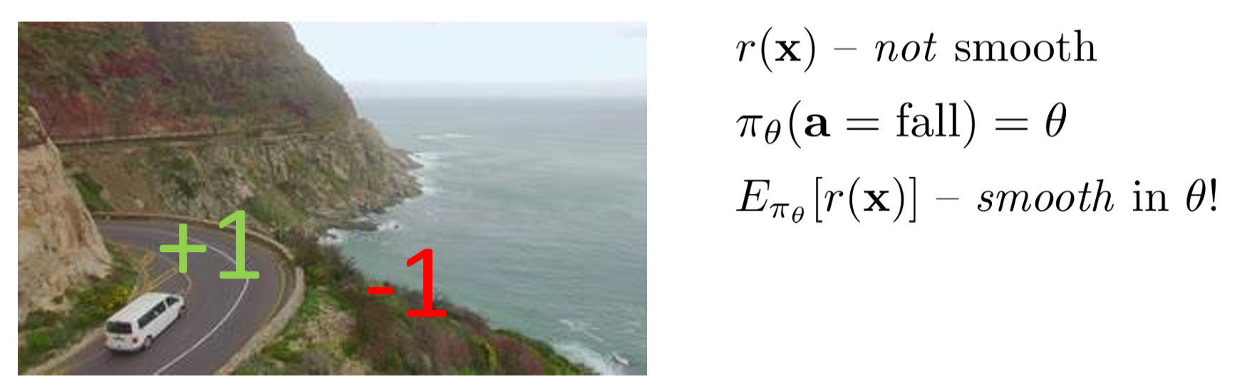
Suppose we are training a self-driving car:

• Safely on the road: Reward +1
• Falls off the cliff: Reward -1

We know that real-world rewards are often not smooth. For instance, the car might be 10 centimeters to the right and still on the road (reward +1); shift just 1 more centimeter to the right, and it falls off the cliff (reward suddenly becomes -1). Such step-function-like discontinuities are non-differentiable. If the function is non-differentiable, your neural network (which relies on backpropagation and gradient descent) is completely blind — it has no idea how to fine-tune the parameters \(\theta\).

We make the policy stochastic. Suppose the neural network outputs a probability of falling off the cliff \(\pi_\theta(\mathbf{a}=\text{fall}) = \theta\). (Here \(\theta\) can be understood as a parameter between 0 and 1.)

Instead of looking at the single-instance reward, we look at the expected reward:

\[ E_{\pi_\theta}[r(\mathbf{x})] = (1-\theta) \cdot (+1) + \theta \cdot (-1) = 1 - 2\theta \]

The originally discontinuous +1 and -1, after being weighted by probability \(\theta\) and summed, become a continuous function (\(1 - 2\theta\)). This function is perfectly smooth, and your neural network can immediately compute the gradient (the derivative is -2), thereby knowing that "to increase the expectation, I must decrease \(\theta\) (the probability of falling off the cliff)."

From this, we can see that the underlying logical chain of reinforcement learning is now complete:

1. Our objective is almost always an expectation, because real-world rewards are discontinuous and non-differentiable. Taking expectations "smooths out" discrete discontinuities, enabling neural networks to compute gradients.
2. The theoretical expectation can be written as a finite-step sum or an infinite-step stationary distribution.
3. Since the theoretical expectation is infeasible to compute exactly, we typically use Monte Carlo sampling to approximate it.

Because real-world rewards are often discontinuous and non-differentiable (e.g., instantly going from +1 to -1 when falling off a cliff), only through probabilistic computation of expectations can we smooth them into continuous mathematical functions, enabling neural networks to compute gradients for parameter updates. In other words, without expectations, neural networks simply cannot learn.

RL Anatomy

Iterative Loop Framework

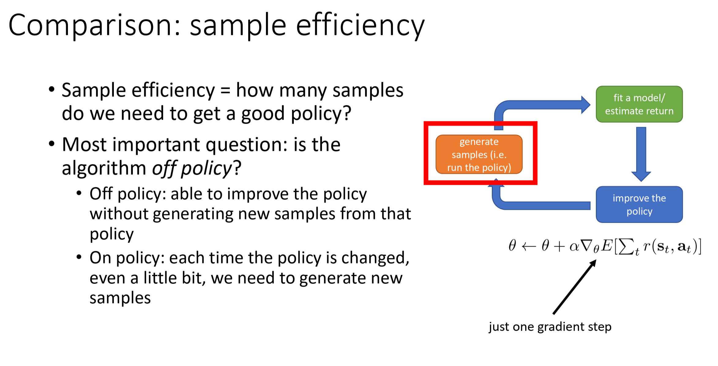
The core architecture (anatomy) of reinforcement learning algorithms can be simplified into a continuously cycling three-step process.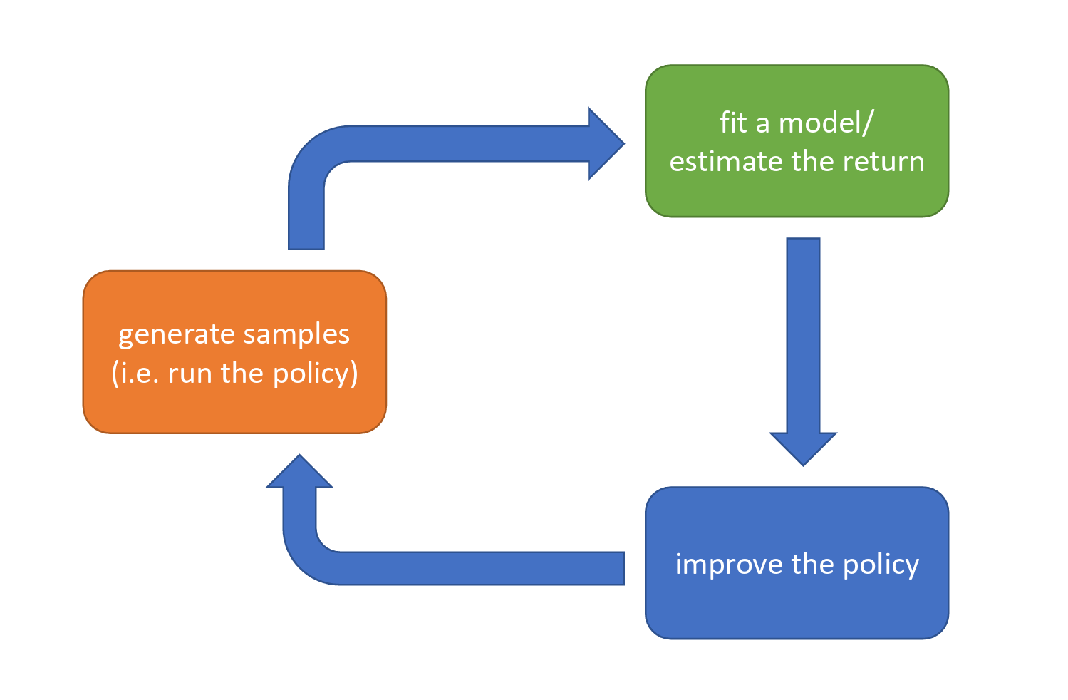

These three steps are:

1. Generate samples — let the agent interact with the environment. The agent makes actions based on the current policy, then collects: states, actions, and rewards.
2. Fit a model / estimate returns — the algorithm evaluates and analyzes the collected data, computing how much reward these actions yielded, or attempting to learn the environment's dynamics (i.e., fitting a model).
3. Improve the policy — based on the evaluation results from the previous step, optimize the agent's behavioral rules. The improved policy will be used in the next round of sample generation, with the goal of making the agent more likely to choose actions that yield higher returns.

RL is an iterative process. The algorithm is not a one-shot procedure but rather continuously evolves through the closed loop of "act -> evaluate -> improve -> act again." Whether it is Deep RL or traditional RL algorithms, they all generally follow this macro-level framework.

Model-Free

Here we briefly introduce model-free RL based on policy gradients. This is just an introduction to illustrate the iterative loop framework.

"Model" in reinforcement learning refers to the agent's understanding of environment dynamics. This understanding typically involves two core questions:

1. State transition: If I am in state \(s\) and take action \(a\), what will the next state \(s'\) be?
2. Reward prediction: How much reward \(r\) will this action give me?

Model-free methods are empiricist in nature — they do not attempt to understand the underlying logic of the environment, but only care about results. Through extensive trial and error, they directly learn "what action to take in what state" (policy) or "how valuable is this state" (value function).

Model-free methods are simple and direct, requiring no complex modeling, and are well-suited for scenarios where the environment is extremely complex and difficult to predict. Their disadvantage is also obvious: low sample efficiency — requiring thousands upon thousands of trials to learn anything useful. Algorithms we learn first when studying RL, such as Q-Learning, SARSA, PPO, and DQN, are all model-free.

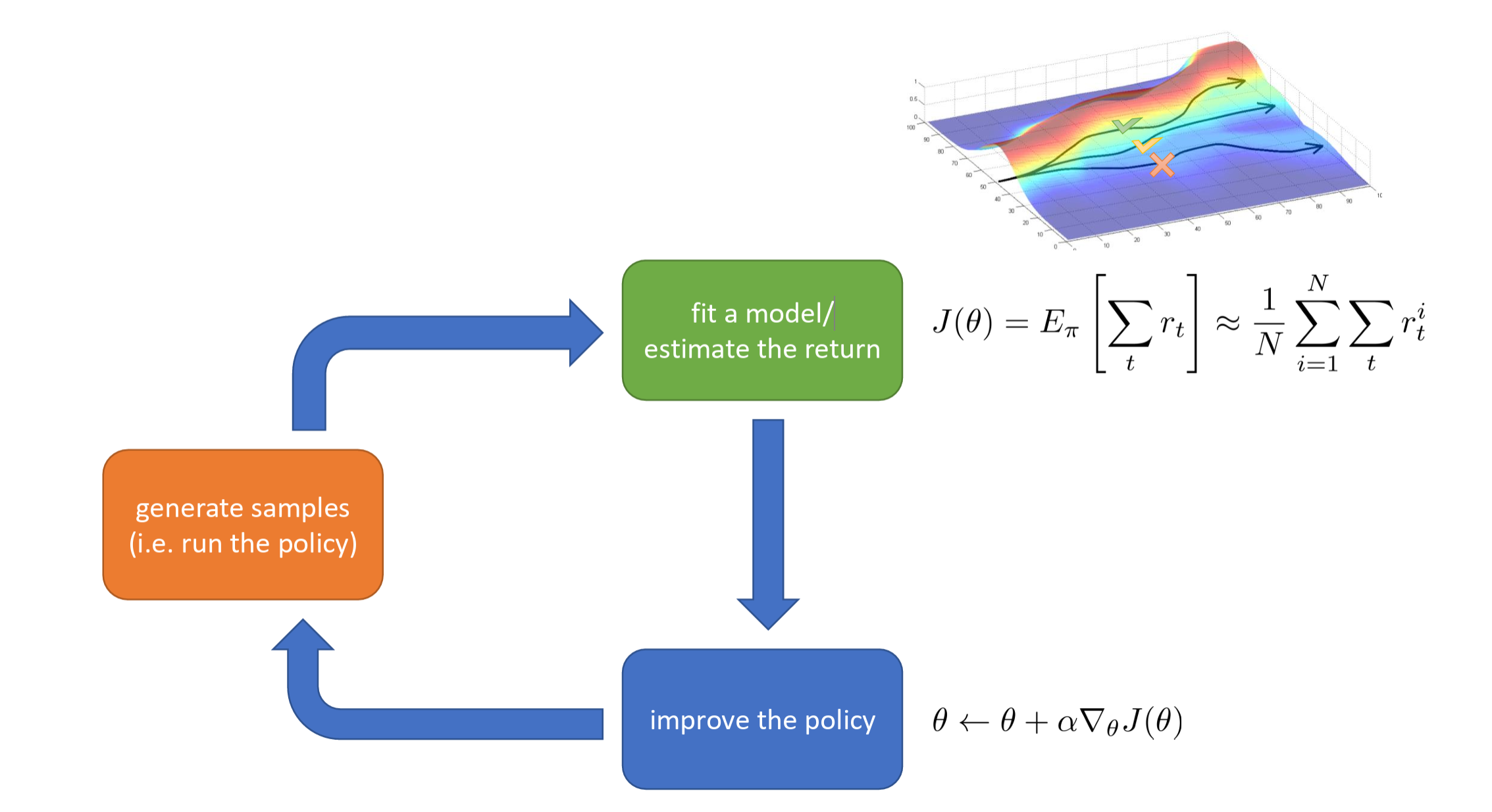
Model-free means we do not care about how the environment works and directly observe outcomes. We directly compute the average total reward over samples:

\[ J(\theta) = E_\pi [\sum r_t] \approx \frac{1}{N} \sum \sum r \]

The formula \(J(\theta) = E_\pi [\sum r_t]\) states that the objective is to maximize the expected return. The right-hand side \(\frac{1}{N} \sum \sum r\) indicates that this expectation is estimated by averaging over multiple experimental trajectories.

We use policy gradient ascent: \(\theta \leftarrow \theta + \alpha \nabla_\theta J(\theta)\) to improve the policy. If a set of actions leads to high reward, increase the probability of producing those actions; if the reward is low, decrease the probability. This is essentially "black-box trial and error."

Model-Based

Model-based methods first attempt to build an "environment simulator" in their heads. The agent tries to learn the rules of the environment. Once it has mastered the rules, it can reason through "imagination" without needing to bump into walls in the real environment every time.

The most common example is Go: a player knows the game rules (model) perfectly — if I place a stone here, the board will look like this. So the player can engage in "deep deliberation" before placing a stone: "If I play A, the opponent might play B, then I follow with C..."

Model-based algorithms include Dyna-Q, AlphaZero, World Models, etc. They are highly sample-efficient, as they can self-practice within the learned model, reducing the danger and cost of interacting with the real environment. Their disadvantage is that if the environment model is wrong (model bias), the agent may go further and further down the wrong path, ultimately performing disastrously in reality.

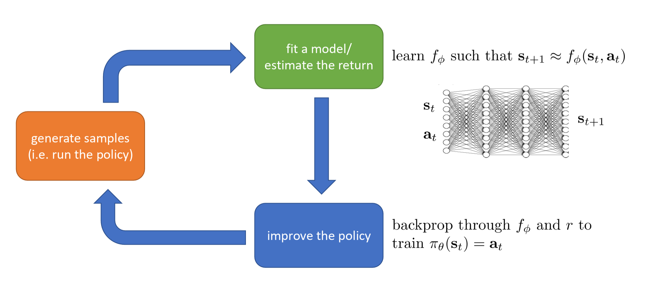
This approach tries to understand the operating principles of the environment — i.e., learn a "world model." It learns a state transition function \(f_\phi\) such that \(s_{t+1} \approx f_\phi(s_t, a_t)\) to fit the model.

The intuition is that it uses a neural network to simulate reality. Given the current state and action as input, it predicts the next state. It is asking: "If I do this, what will the world become?"

Then, it improves the policy through backpropagation through the model and reward function. Because it now has a differentiable model \(f_\phi\), it can directly compute "how small changes in actions affect future states and consequently affect rewards." This is more precise than the "trial and error" approach, because it leverages the internal logic of the environment.

Two-Level Loop

Modern RL combines Model-Free and Model-Based ideas, using a two-level loop approach: one layer interacts with the real world, and the other reasons within the "mind."

These are relatively recent methods, and the specific implementation details and approaches will be supplemented later.

Cost Assessment

In the RL Anatomy, the costs of each component are as follows:

1. The time cost of generating samples is high. If running on real robots, autonomous vehicles, or power grids, physical laws constrain operations to "real-time." This means collecting 1 hour of data actually takes 1 hour. This is a significant time cost in both research and industrial applications. If high-performance simulators are available, speed can increase to 10,000x faster than the real world, greatly alleviating this cost.
2. The computational cost of fitting models / estimating returns is high.
3. The cost of improving the policy is typically not the bottleneck compared to the above two.

We can observe that the main bottlenecks in reinforcement learning are:

1. Time cost of data acquisition
2. Computational cost of model training

Value Estimation and Policy Improvement

Q-function

The Q-function, formally called the State-Action Value Function, is typically denoted \(Q(s, a)\). Its core purpose is to evaluate how good it is to take a particular action in a specific state. Specifically, when you are in state \(s\), choose action \(a\), and subsequently follow a specific policy, \(Q(s, a)\) represents the expected cumulative total reward you can obtain from now until the end.

We know that the original objective of reinforcement learning is:

\[ E_{\tau \sim p_\theta(\tau)} \left[ \sum_{t=1}^H r(\mathbf{s}_t, \mathbf{a}_t) \right] \]

It represents the expectation of the sum of all single-step rewards \(r\) along a trajectory \(\tau\) of length \(H\) generated under policy \(\theta\). This is a global, macroscopic objective over the entire timeline, and directly optimizing it is very difficult.

A long trajectory can actually be decomposed into two parts: the first step's return + all future steps' return.

\[ Q(\mathbf{s}_1, \mathbf{a}_1) = r(\mathbf{s}_1, \mathbf{a}_1) + E_{\mathbf{s}_2 \sim p} \left[ E_{\mathbf{a}_2 \sim \pi} [r(\mathbf{s}_2, \mathbf{a}_2) + ... | \mathbf{s}_2] | \mathbf{s}_1, \mathbf{a}_1 \right] \]

This formally defines the Q function. It asks: "What if we already knew the expected return from the future (the part enclosed in braces)?" In this way, the Q function compresses the complex future from step 2 to step \(H\) into a single known value.

\[ E_{\tau \sim p_\theta(\tau)} \left[ \sum_{t=1}^H r(\mathbf{s}_t, \mathbf{a}_t) \right] = E_{\mathbf{s}_1 \sim p(\mathbf{s}_1)} \left[ E_{\mathbf{a}_1 \sim \pi(\mathbf{a}_1|\mathbf{s}_1)} [Q(\mathbf{s}_1, \mathbf{a}_1)|\mathbf{s}_1] \right] \]

By substituting the Q function, the originally massive objective that requires considering the entire long trajectory \(\tau\) (left side) is equivalently replaced by an extremely simple objective that only considers the first step's state and action (right side). All "future predictions" are packaged inside \(Q(\mathbf{s}_1, \mathbf{a}_1)\).

If we truly knew the perfect Q function, then policy improvement would become trivially simple. We would not need to reason hundreds of steps ahead — we would just look at which action \(\mathbf{a}_1\) has the highest Q value (i.e., \(\arg\max\)) and choose that action with 100% probability (this is the greedy policy).

Here is a more rigorous definition:

\[ Q^\pi(\mathbf{s}_t, \mathbf{a}_t) = \sum_{t'=t}^T E_{\pi_\theta}[r(\mathbf{s}_{t'}, \mathbf{a}_{t'}) | \mathbf{s}_t, \mathbf{a}_t] \]

In state \(\mathbf{s}_t\), you forcibly take the specific action \(\mathbf{a}_t\), and from that point on follow the policy \(\pi_\theta\) until time \(T\), the "expected total reward" you can obtain.

Chess analogy: The current board position is \(\mathbf{s}_t\). The Q function evaluates: "If I move my knight to f3 (action \(\mathbf{a}_t\)) this turn", and then play the rest of the game at my normal level, what is my probability of winning or my expected score? It specifically assesses the quality of a particular action.

Value Function

The value function (state value function) is typically denoted \(V\):

\[ V^\pi(\mathbf{s}_t) = \sum_{t'=t}^T E_{\pi_\theta}[r(\mathbf{s}_{t'}, \mathbf{a}_{t'}) | \mathbf{s}_t] \]

When in state \(\mathbf{s}_t\), if you follow policy \(\pi_\theta\) from now until the end, the "expected total reward" you can obtain. Note that here, no specific first action is mandated — the action is chosen entirely according to the policy \(\pi_\theta\), whether stochastically or deterministically.

Chess analogy: The current board position is \(\mathbf{s}_t\). The V function evaluates: "Is this position favorable or unfavorable for me?" (e.g., the common "White has an advantage: +2.0"). It assesses only the quality of the state itself, without specifying any particular move.

---

The value of a state (\(V\)) equals the weighted average of the values (\(Q\)) of all possible actions in that state. The weights are the probabilities assigned by the policy \(\pi\) to choosing each action.

\[ V^\pi(\mathbf{s}_t) = E_{\mathbf{a}_t \sim \pi(\mathbf{a}_t|\mathbf{s}_t)}[Q^\pi(\mathbf{s}_t, \mathbf{a}_t)] \]

In other words, how good a situation is depends on how good the various moves available in that situation are, and how likely you are to choose those good moves.

Two Core Formulas of RL

From the above, it is not hard to deduce that the ultimate goal of reinforcement learning is to maximize the expected value of the initial state \(\mathbf{s}_1\)****, namely:

\[ E_{\mathbf{s}_1 \sim p(\mathbf{s}_1)}[V^\pi(\mathbf{s}_1)] \text{ is the RL objective!} \]

So after we compute the Q function and V function, how exactly should we use them to make the AI smarter (improve the policy)?

There are generally two mainstream approaches:

1. Greedy policy improvement — i.e., value-based methods
2. Increasing the probability of good actions — i.e., policy gradient methods

For the first approach — greedy policy improvement, also known as "value-based" methods (such as Q-learning, DQN) — if we have an old policy \(\pi\) and have computed the corresponding \(Q^\pi(\mathbf{s}, \mathbf{a})\), we can easily obtain a better new policy \(\pi'\). The method is simple: in state \(\mathbf{s}\), whichever action \(\mathbf{a}\) has the highest Q value (i.e., \(\arg\max_{\mathbf{a}} Q^\pi(\mathbf{s}, \mathbf{a})\)), we set the probability of taking that action to 1 (i.e., choose it with 100% certainty). This is a "simple but effective" improvement approach. Since the Q function already tells you the future score for each action, there is no need to hesitate — just always pick the action with the highest score. It can be mathematically proven that the new policy \(\pi'\) constructed this way is at least as good as the old policy \(\pi\), and usually better (this policy is at least as good as \(\pi\) (and probably better)!). This forms a closed loop: evaluate policy -> select max Q value to improve policy -> re-evaluate -> improve again, until the policy is optimal.

The core policy update formula for this approach is:

\[ \pi'(\mathbf{a}|\mathbf{s}) = 1 \quad \text{if} \quad \mathbf{a} = \arg\max_{\mathbf{a}} Q^\pi(\mathbf{s}, \mathbf{a}) \]

Under the new policy \(\pi'\), in state \(\mathbf{s}\), if action \(\mathbf{a}\) maximizes the corresponding \(Q\) value, we execute it with probability \(1\) (i.e., \(100\%\)), and all other actions have probability \(0\).

---

For the second approach — increasing the probability of good actions (Policy Gradient), also known as "policy gradient" methods (such as REINFORCE, Actor-Critic, PPO) — we compute gradients to increase the probability of "good actions" being selected. How do we define whether an action is good? If \(Q^\pi(\mathbf{s}, \mathbf{a}) > V^\pi(\mathbf{s})\), it means action \(\mathbf{a}\) is better than average. Therefore, we should modify the policy \(\pi(\mathbf{a}|\mathbf{s})\) to increase the probability of selecting this action:

• If a specific action's score \(Q\) is greater than the average score \(V\), it means this action is an "above-average" good action, and in future training we should encourage the AI to take this action more often (increase probability).
• Conversely, if \(Q < V\), it means this action is "dragging things down," and we should penalize it by reducing its selection probability.

The difference \(Q^\pi(\mathbf{s}, \mathbf{a}) - V^\pi(\mathbf{s})\) has a dedicated term in reinforcement learning: the Advantage Function, typically denoted \(A(\mathbf{s}, \mathbf{a})\). It measures "how much better this action is compared to the average."

The core formula for this approach is the advantage function:

\[ A^\pi(\mathbf{s}, \mathbf{a}) = Q^\pi(\mathbf{s}, \mathbf{a}) - V^\pi(\mathbf{s}) \]

The policy update logic is:

• If \(A^\pi(\mathbf{s}, \mathbf{a}) > 0\) (i.e., \(Q^\pi > V^\pi\)): Action \(\mathbf{a}\) is a "good action," and in future policy updates we need to increase the probability \(\pi(\mathbf{a}|\mathbf{s})\).
• If \(A^\pi(\mathbf{s}, \mathbf{a}) < 0\) (i.e., \(Q^\pi < V^\pi\)): Action \(\mathbf{a}\) is a "bad action," and in future policy updates we need to decrease the probability \(\pi(\mathbf{a}|\mathbf{s})\).

---

These two core formulas are extremely important in RL, and we will encounter them repeatedly in our subsequent studies.

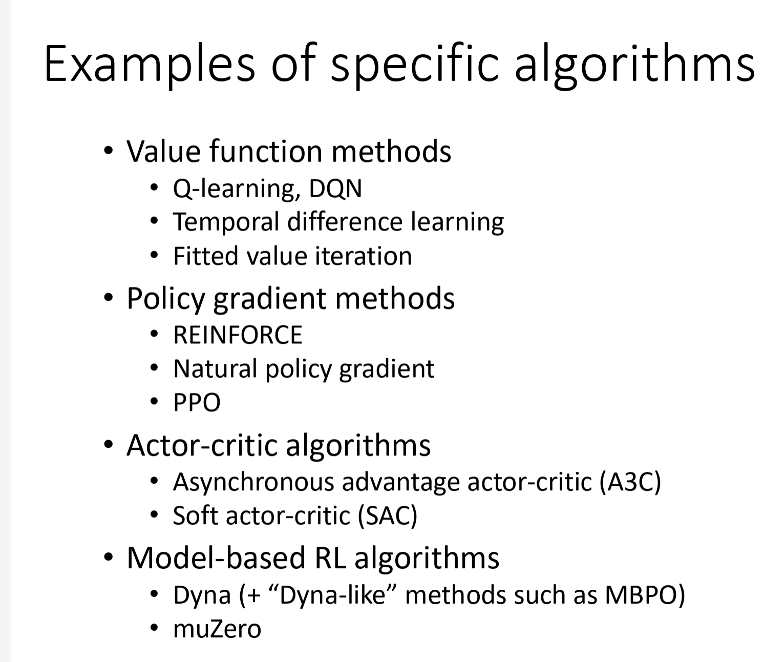
RL Algorithm Types

The core objective of all RL algorithms is to maximize expected return:

\[ \theta^\star = \arg\max_\theta E_{\tau \sim p_\theta(\tau)} \left[ \sum_t r(\mathbf{s}_t, \mathbf{a}_t) \right] \]

Let us briefly survey the major algorithm types and their key differences. We will explore specific algorithms in greater depth in future study.

Value-based

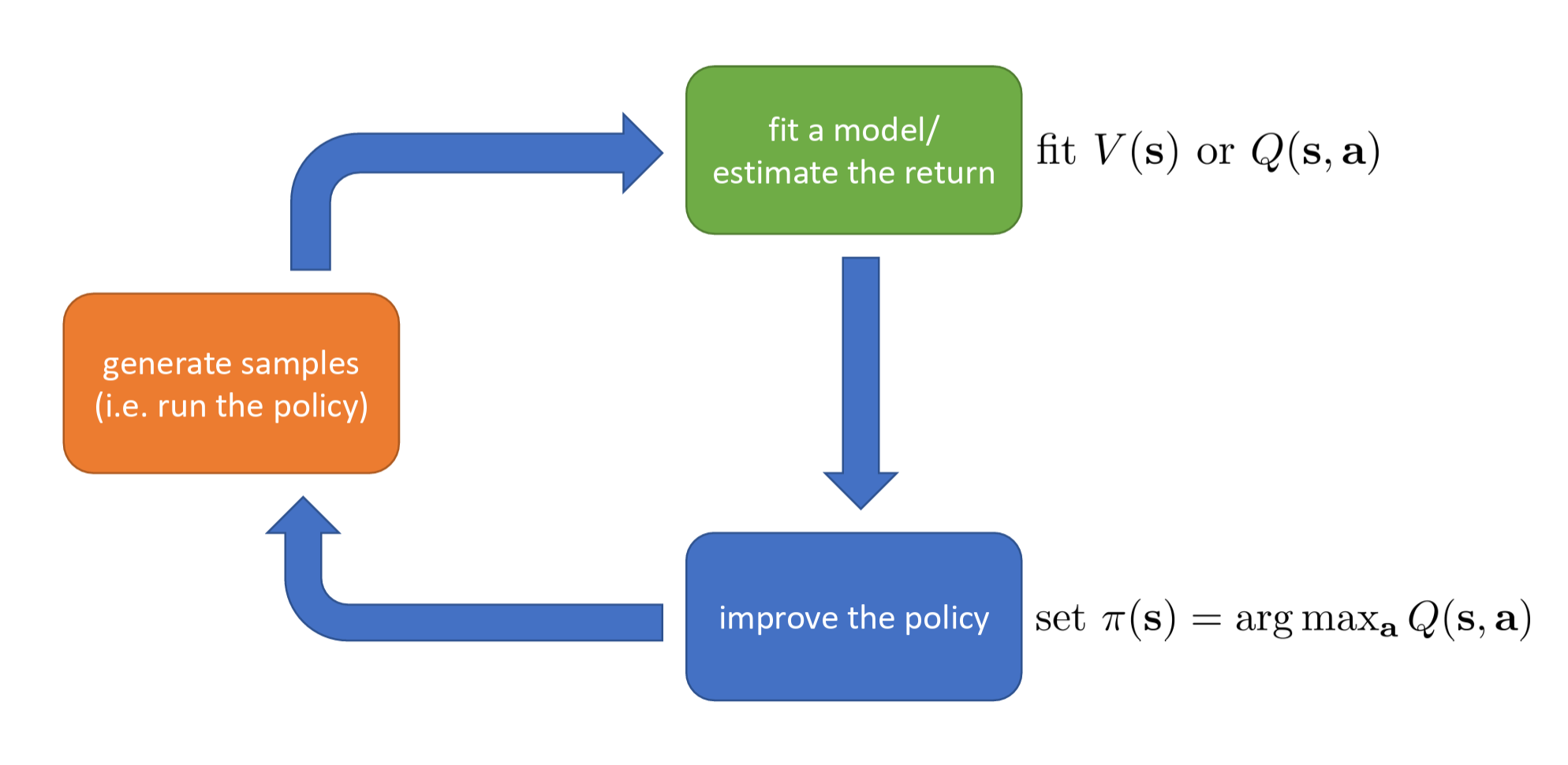
Value-based estimate value function or Q-function of the optimal policy (no explicit policy).

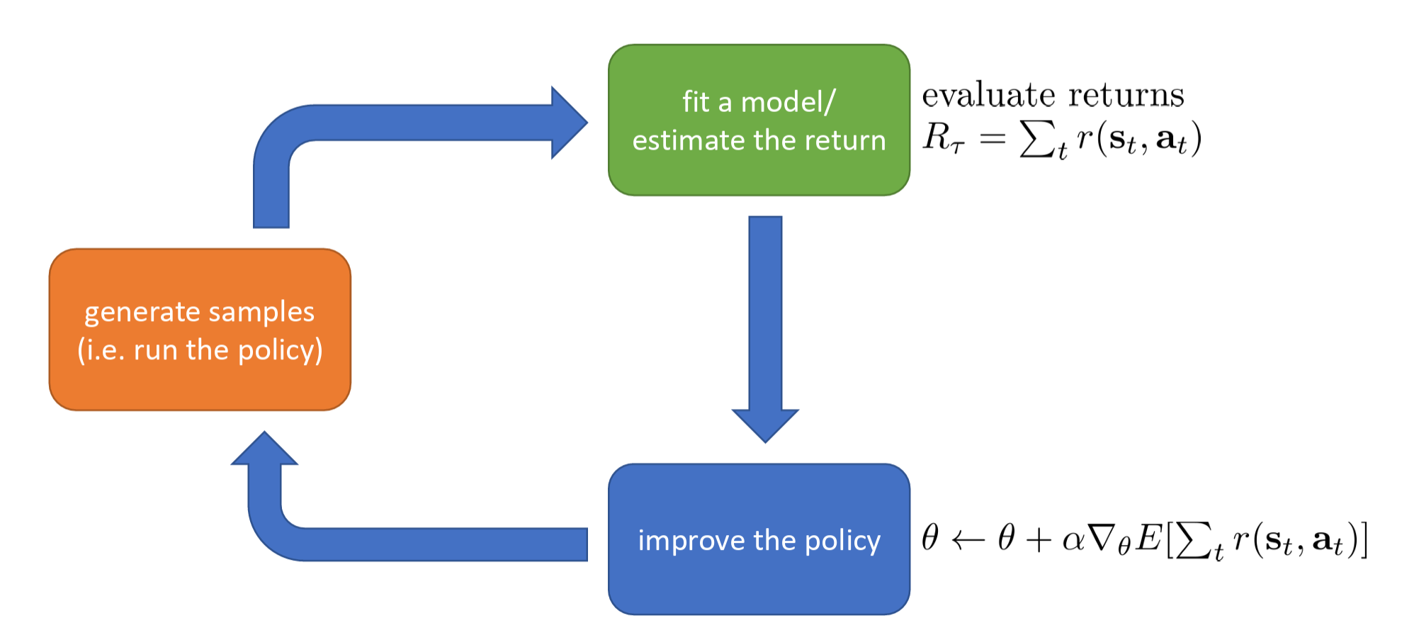
Policy Gradients

Policy gradients directly differentiate the above objective.

Actor-Critic

Actor-critic estimate value function or Q-function of the current policy, use it to improve policy.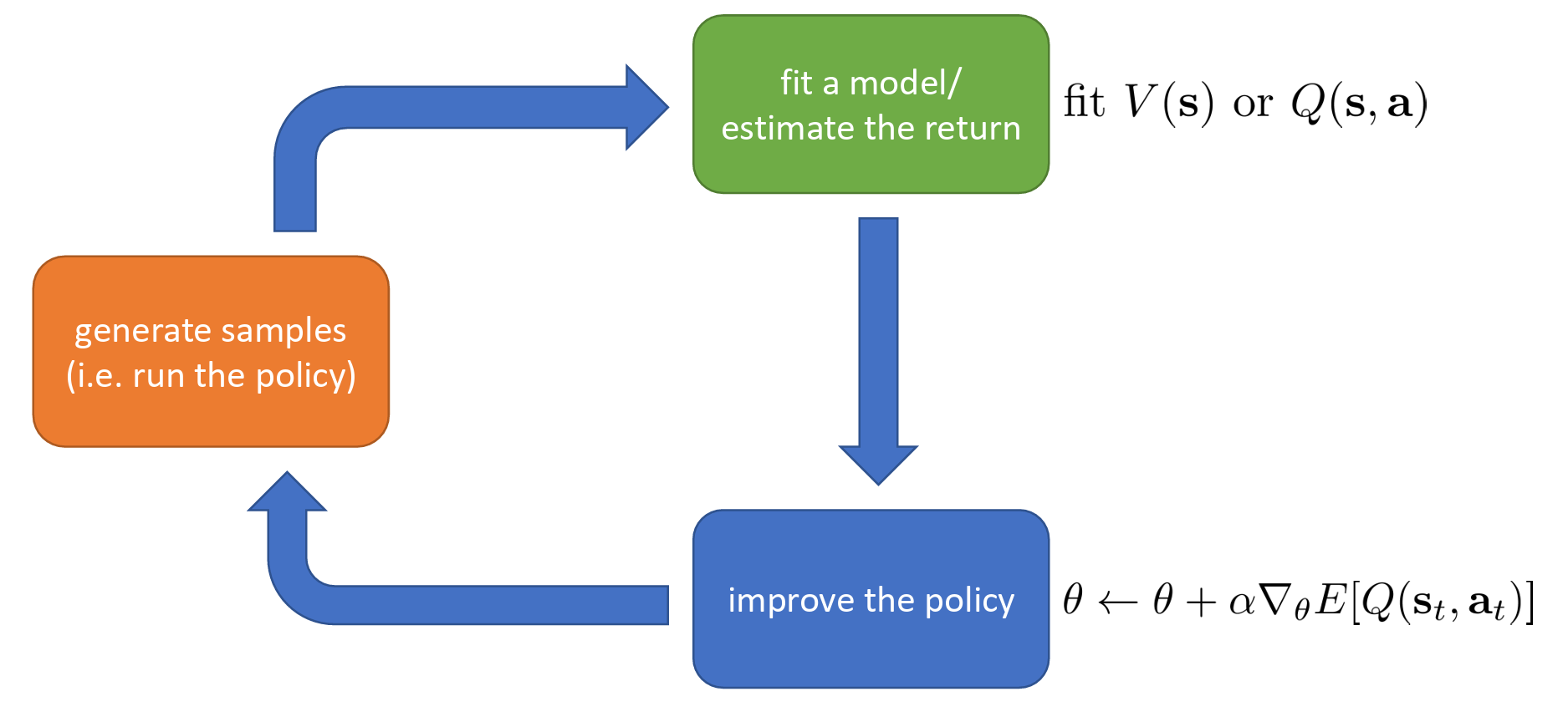

Model-based

Model-based RL estimate the transition model, and then use it for planning (no explicit policy), use it to improve a policy, and something else.

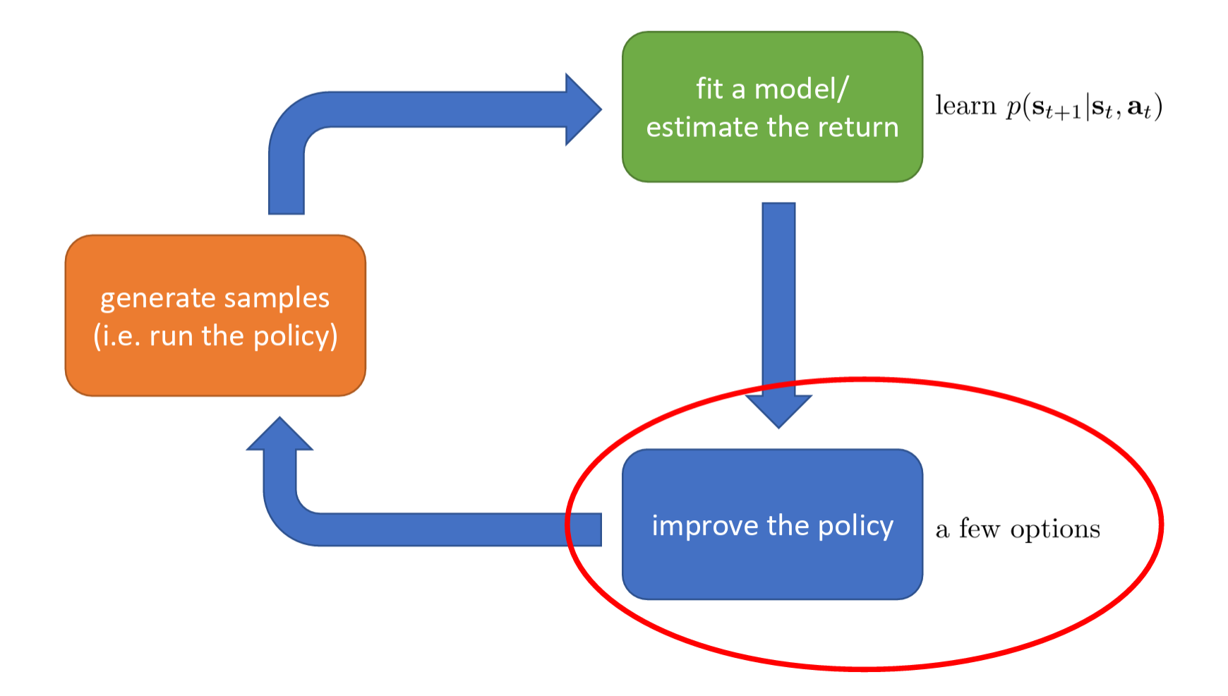
improve the policy — a few options

1. Just use the model to plan (no policy) • Trajectory optimization / optimal control (primarily in continuous spaces) – essentially backpropagation to optimize over actions • Discrete planning in discrete action spaces – e.g., Monte Carlo tree search
2. Backpropagate gradients into the policy • Requires some tricks to make it work
3. Use the model to learn a value function • Dynamic programming • Generate simulated experience for model-free learner

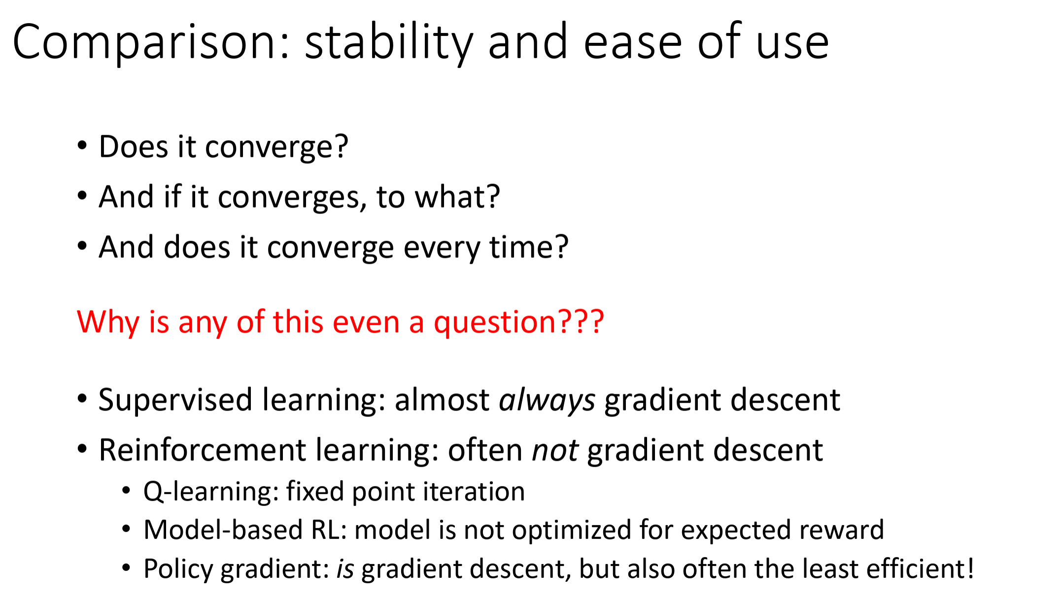
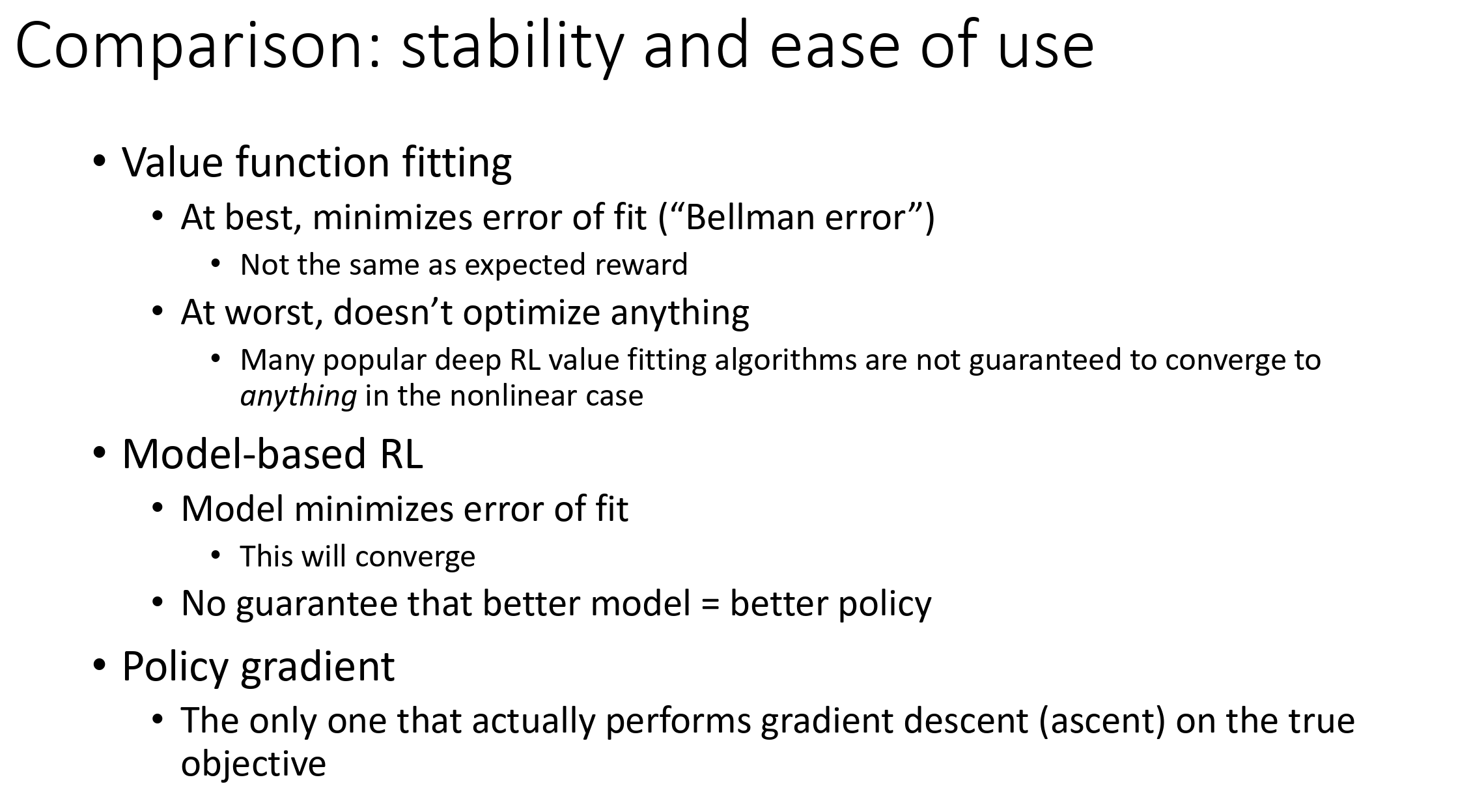
Comparison

The reason so many RL algorithms exist is that different tasks involve different tradeoffs and different assumptions:

1. Different tradeoffs: Sample Efficiency / Stability & ease of use
2. Different assumptions: Stochastic or Deterministic? / Continuous or discrete? / Episodic or infinite horizon?
3. Easier to represent the policy? / Easier to represent the model?

---

评论