Transformer
Given that the Transformer architecture has gradually become the core architecture of deep learning and even machine learning as a whole, I have dedicated this separate note to document my study of the Transformer architecture. In the DNN architecture overview, we briefly touched on some characteristics of Transformers; in this note, we will explore them in much greater depth.
From RNN/CNN to Transformer
As we saw in the RNN notes, RNNs suffer from two critical problems:
| Problem | RNN's Dilemma | Transformer's Solution |
|---|---|---|
| No parallelism | \(h_t\) must wait for \(h_{t-1}\), sequential dependency \(O(n)\) | Self-Attention processes all positions at once, \(O(1)\) sequential operations |
| Long-range dependencies | Gradients vanish after many multiplicative steps, failing to retain distant information | Any two positions are directly connected with path length \(O(1)\) |
LSTM/GRU alleviated gradient vanishing but could not solve the parallelism problem. The Attention mechanism was originally introduced as an auxiliary component for Seq2Seq (Bahdanau, 2014), but in 2017 Vaswani et al. proposed a radical idea: discard RNNs entirely and build the whole model using only Attention.
"Attention is All You Need" — Vaswani et al., 2017
Architecture Overview
Full Architecture Diagram
The figure below shows the complete Transformer architecture (source: "Attention Is All You Need" original paper):
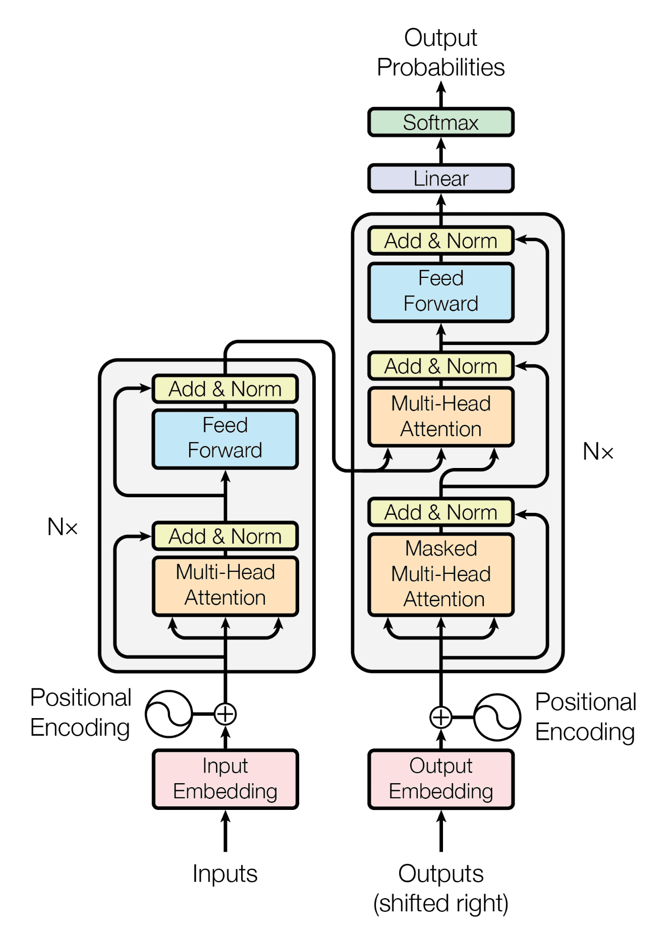
Key architectural points:
- Left half = Encoder: processes the source language input and outputs a contextual representation for each token
- Right half = Decoder: leverages the Encoder's output to autoregressively generate the target language
- Nx denotes stacking \(N\) layers (original paper: \(N=6\))
- Core hyperparameters: \(d_{\text{model}}=512\), \(h=8\) heads, \(d_{ff}=2048\)
Data Flow: A Complete Translation Pass
Taking the translation of "我 喜欢 猫" → "I like cats" as an example:
- Input encoding: Source sentence "我 喜欢 猫" → Token Embedding + Positional Encoding
- Encoder processing: Passes through 6 Encoder layers, each performing Self-Attention + FFN, ultimately producing a contextual representation for every source token
- Decoder autoregressive generation:
- Input
<BOS>(beginning-of-sentence token) → Decoder attends to Encoder output via Cross-Attention → predicts "I" - Input
<BOS> I→ predicts "like" - Input
<BOS> I like→ predicts "cats" - Input
<BOS> I like cats→ predicts<EOS>(end-of-sentence token)
- Input
Input Processing
Token Embedding
Maps discrete words (tokens) to continuous vectors. This is similar to Word2Vec, but the Transformer's embedding matrix is trained jointly with the model.
where \(E \in \mathbb{R}^{V \times d_{\text{model}}}\) is the embedding matrix and \(V\) is the vocabulary size.
Note: The original paper scales the embedding vectors by \(\sqrt{d_{\text{model}}}\):
This ensures that the embedding and Positional Encoding remain on a comparable scale when added together.
Positional Encoding
Why do we need positional encoding?
Self-Attention is a set operation — it processes inputs regardless of their order. Without positional information, "dog bites man" and "man bites dog" would be identical to the model. Positional Encoding injects ordering information into each position.
Sinusoidal positional encoding:
- \(pos\): position of the token in the sequence (0, 1, 2, ...)
- \(i\): dimension index (0, 1, ..., \(d_{\text{model}}/2 - 1\))
- Even dimensions use \(\sin\), odd dimensions use \(\cos\)
Intuitive understanding: Each dimension corresponds to a "pendulum" oscillating at a different frequency. Low dimensions change rapidly (high frequency), while high dimensions change slowly (low frequency). This is analogous to a binary counter — the least significant bit flips fastest, and the most significant bit flips slowest. The combination at each position is unique, just as every number has a unique binary representation.
Why use sine/cosine rather than simple linear encoding (e.g., 1, 2, 3...)?
- Boundedness: Values stay within \([-1, 1]\), preventing explosion as position increases
- Learnable relative positions: For a fixed offset \(k\), \(PE_{pos+k}\) can be expressed as a linear function of \(PE_{pos}\) (via trigonometric sum-to-product identities), enabling the model to learn relative positional relationships:
where \(\omega = 1/10000^{2i/d_{\text{model}}}\). In other words, the encoding at position \(pos+k\) can be obtained from the encoding at position \(pos\) through a linear transformation that depends only on \(k\) (not on \(pos\)).
- Extrapolation: In theory, it can generalize to sequence lengths unseen during training
How it combines with the input: Direct addition (not concatenation)
Encoder in Detail
The figure below highlights the Encoder portion (within the red box):
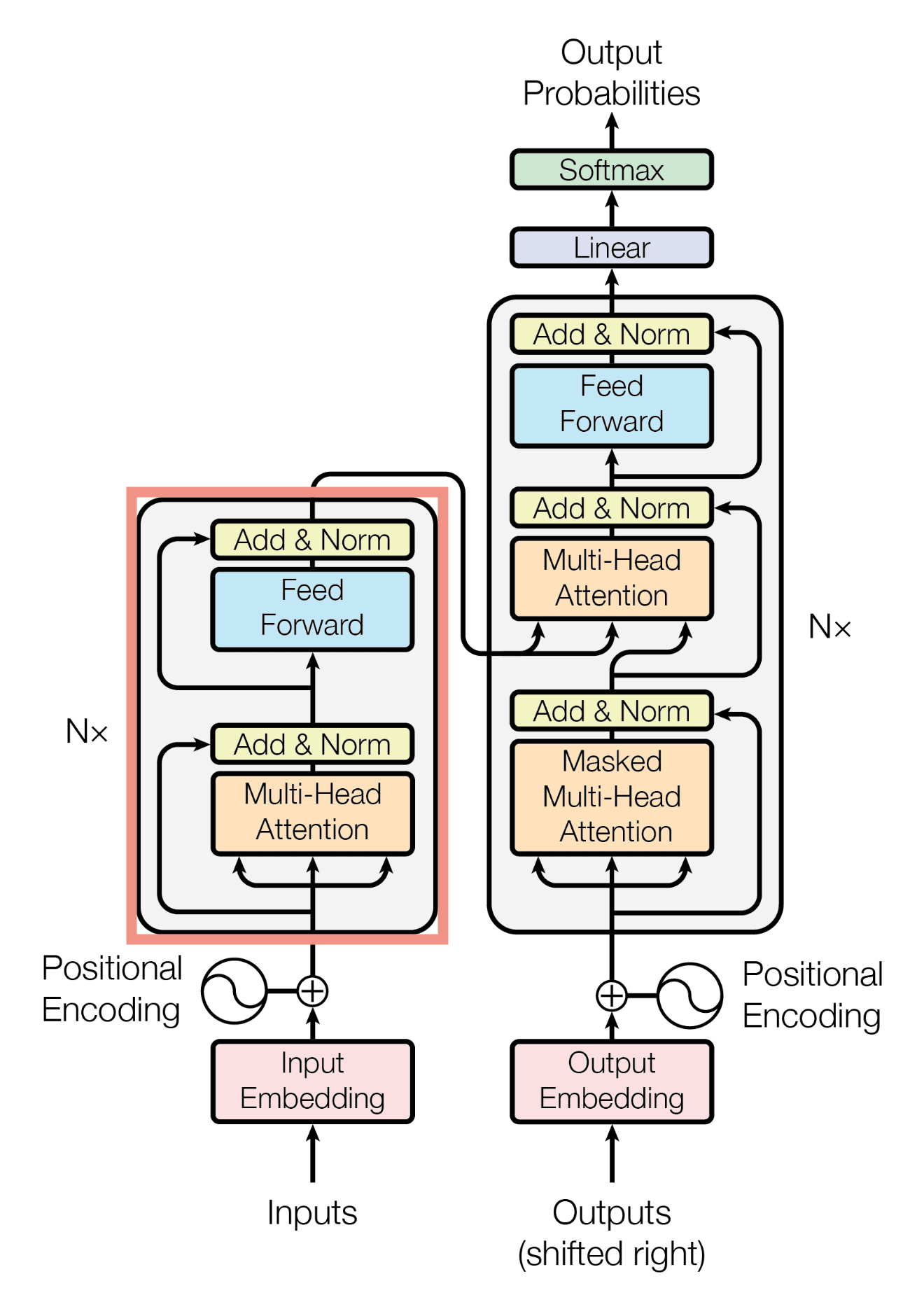
Each Encoder layer contains two sub-layers: Multi-Head Self-Attention and Feed-Forward Network, each wrapped with a residual connection + Layer Normalization.
Sub-layer 1: Multi-Head Self-Attention
Self-Attention in the Encoder allows every source token to attend to all other source tokens, building a global contextual understanding.
The figure below illustrates the internal structure of Scaled Dot-Product Attention and Multi-Head Attention (source: original paper):
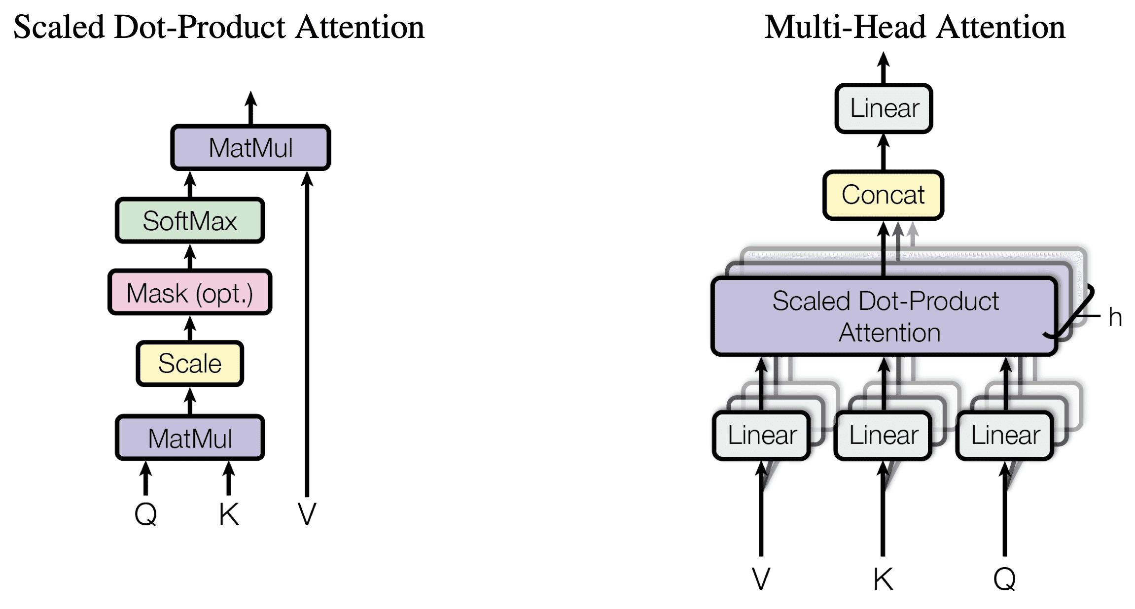
Scaled Dot-Product Attention (left) computation flow:
- MatMul: Multiply \(Q\) and \(K^T\) to obtain the attention score matrix \(\in \mathbb{R}^{n \times n}\)
- Scale: Divide by \(\sqrt{d_k}\) to prevent large dot products from pushing softmax into regions with vanishing gradients
- Mask (optional): Causal mask in the Decoder, setting future positions to \(-\infty\)
- Softmax: Normalize scores into a probability distribution (each row sums to 1)
- MatMul: Compute a weighted sum of \(V\) using the attention weights to produce the output
Multi-Head Attention (right) computation flow:
- \(h=8\) heads, each with dimension \(d_k = d_v = d_{\text{model}} / h = 64\)
- Each head learns a different attention pattern (e.g., syntactic relations, semantic relations, positional relations, etc.)
- The outputs are concatenated and projected back to \(d_{\text{model}}\) dimensions through a linear layer \(W^O\)
When encoding "我 吃 苹果" (I eat apple):
- "苹果" (apple) can attend to "吃" (eat), understanding that "苹果" here refers to a fruit (not the company)
- "吃" (eat) can attend to "我" (I), understanding the subject of the action
This answers the question posed for reflection: "When translating '苹果' (apple), does the model actually attend to the preceding verb '吃' (eat)?" — Yes. Self-Attention allows "苹果" to directly attend to "吃" with \(O(1)\) path length, dynamically adjusting its representation based on context.
Sub-layer 2: Position-wise Feed-Forward Network (FFN)
Applies the same two-layer fully connected network independently to each position:
Or written more explicitly as two steps:
- \(W_1 \in \mathbb{R}^{d_{\text{model}} \times d_{ff}}\): projects up, \(512 \to 2048\)
- \(W_2 \in \mathbb{R}^{d_{ff} \times d_{\text{model}}}\): projects down, \(2048 \to 512\)
Why is the FFN needed?
Self-Attention is a linear weighted summation operation (softmax weights × Value). Even when stacked across multiple layers, it only performs weighted combinations. The FFN introduces non-linearity (via ReLU), granting the model non-linear transformation capability.
What "position-wise" means: The FFN is applied independently to each position in the sequence, with no interaction between positions. Information exchange across positions is handled entirely by Self-Attention. You can think of the FFN as each token's "independent reasoning," while Self-Attention is the "discussion and communication" among tokens.
Residual Connection and Layer Normalization
Each sub-layer is equipped with a residual connection and layer normalization:
Residual connection (He et al., 2015): Allows gradients to "skip over" the sub-layer and propagate directly, addressing the gradient vanishing problem in deep networks.
If the transformation learned by \(f(x)\) is poor, gradients can at least flow back through the identity mapping \(x\).
Layer Normalization: Normalizes across the feature dimension of a single sample:
- \(\mu = \frac{1}{d}\sum_{i=1}^d x_i\): mean across the feature dimension
- \(\sigma^2 = \frac{1}{d}\sum_{i=1}^d (x_i - \mu)^2\): variance across the feature dimension
- \(\gamma, \beta\): learnable scale and shift parameters
- \(\epsilon\): small constant to prevent division by zero
Why Layer Norm Instead of Batch Norm?
This answers one of the questions posed for reflection.
Batch Norm: Normalizes across the batch dimension (for a given feature, computes mean and variance across all samples in the batch)
Layer Norm: Normalizes across the feature dimension (for a given sample, computes mean and variance across all features)
              Batch Norm              Layer Norm
              跨样本归一化             跨特征归一化

Batch:  ┌ Sample1: [f1 f2 f3 f4] ┐   Sample1: [f1 f2 f3 f4] ← 在这一行归一化
        │ Sample2: [f1 f2 f3 f4] │   Sample2: [f1 f2 f3 f4] ← 在这一行归一化
        │ Sample3: [f1 f2 f3 f4] │   Sample3: [f1 f2 f3 f4] ← 在这一行归一化
        └────────────────────────┘
              ↑  在每一列归一化
Three reasons Layer Norm is better suited for NLP:
- Variable-length sequences: In NLP, each sample has a different sequence length. Batch Norm requires statistics across samples, but the 10th position in different samples may have entirely different semantic roles, making such statistics meaningless.
- Small batch issue: Transformer training often uses small batch sizes (due to GPU memory constraints), leading to unstable Batch Norm statistics.
- No batch dependency at inference: Layer Norm only looks at the individual sample, so its behavior at inference is identical to training — no need to maintain running mean/variance.
Decoder in Detail
The figure below highlights the Decoder portion (within the red box):
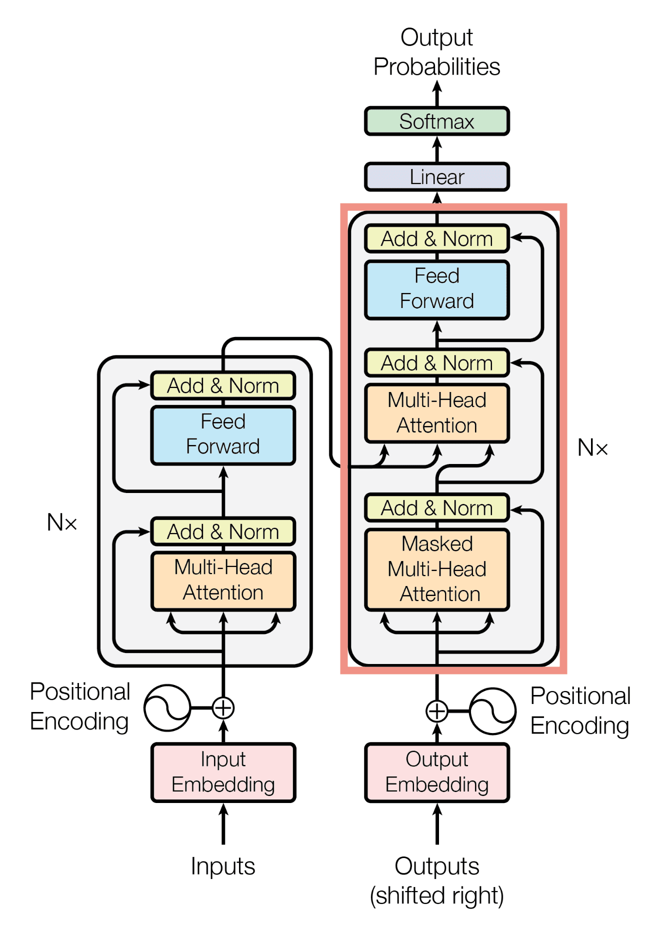
The Decoder has one more sub-layer than the Encoder, for a total of three sub-layers:
Sub-layer 1: Masked Multi-Head Self-Attention
Nearly identical to the Encoder's Self-Attention, with the sole difference being the addition of a causal mask:
Why is the mask needed?
During training, the Decoder sees the complete target sequence (e.g., "I like cats"), but to simulate the autoregressive generation process, generating the \(t\)-th token must not "peek" at tokens \(t+1, t+2, \ldots\).
目标序列: <BOS> I like cats <EOS>

生成 "I"    时,只能看到 <BOS>
生成 "like" 时,只能看到 <BOS> I
生成 "cats" 时,只能看到 <BOS> I like
生成 <EOS>  时,只能看到 <BOS> I like cats

掩码矩阵(0=可见,-∞=遮蔽):
         <BOS>  I    like  cats  <EOS>
<BOS>  [  0    -∞    -∞    -∞    -∞  ]
I      [  0     0    -∞    -∞    -∞  ]
like   [  0     0     0    -∞    -∞  ]
cats   [  0     0     0     0    -∞  ]
<EOS>  [  0     0     0     0     0  ]
This mask is added to the attention scores before softmax. \(-\infty\) becomes 0 after softmax, effectively blocking information flow.
Key to training efficiency: With the mask, the Decoder can process the entire target sequence in parallel at once (rather than generating step by step like an RNN), because the mask ensures each position only sees the history it is supposed to see. This is known as Teacher Forcing.
Sub-layer 2: Cross-Attention (Encoder-Decoder Attention)
This is the bridge connecting the Encoder and the Decoder:
- Query comes from the current Decoder layer's output ("What am I trying to translate?")
- Key and Value come from the Encoder's final output ("What did the source language say?")
This allows the Decoder, when generating each target token, to attend to the most relevant parts of the source language. For example, when generating "cats," Cross-Attention assigns high weight to the Encoder output corresponding to "猫."
Sub-layer 3: Feed-Forward Network
Identical to the FFN in the Encoder.
Output Layer
The output from the top Decoder layer passes through a linear layer + softmax to produce a probability distribution over the vocabulary:
\(W_{\text{vocab}} \in \mathbb{R}^{V \times d_{\text{model}}}\); in practice, this is typically weight-tied with the Token Embedding matrix to reduce the number of parameters.
Forward Pass: A Complete Numerical Example
Following the style of the RNN and CNN notes, we walk through the entire Transformer forward pass using a concrete numerical example.
For simplicity, we use a minimal Transformer: \(d_{\text{model}}=4\), \(h=2\) (2 heads), \(d_k = d_v = 2\), \(d_{ff}=8\), \(N=1\) (1 layer), vocabulary size \(V=6\).
Translation task: "我 猫" → "I cat"
Step 1: Input Embedding + Positional Encoding
Token Embedding (looked up from embedding matrix \(E\)):
Positional Encoding (computed using the sinusoidal formula):
Sum to obtain Encoder input:
Input matrix \(X \in \mathbb{R}^{2 \times 4}\) (2 tokens, each 4-dimensional):
Step 2: Encoder Self-Attention
Generate Q, K, V (via linear transformations \(W^Q, W^K, W^V \in \mathbb{R}^{4 \times 4}\)):
Split into 2 heads (each head has \(d_k = 2\)):
where \(Q_1, K_1, V_1 \in \mathbb{R}^{2 \times 2}\) (first 2 columns), \(Q_2, K_2, V_2 \in \mathbb{R}^{2 \times 2}\) (last 2 columns).
Head 1 Attention computation:
(a) Attention scores:
Suppose the result is:
(b) Softmax (normalized per row):
How to interpret the attention weights
Row 1 \([0.60, 0.40]\) means "我" attends 60% to itself and 40% to "猫." Row 2 \([0.35, 0.65]\) means "猫" attends 35% to "我" and 65% to itself.
(c) Weighted sum:
Head 2 is computed analogously, yielding \(\text{head}_2 \in \mathbb{R}^{2 \times 2}\).
Concatenation + linear transformation:
Step 3: Residual Connection + Layer Norm
For each token vector (each row): compute mean \(\mu\) and variance \(\sigma^2\), then normalize.
Suppose "我" after Attention yields \([0.3, 0.7, 0.5, 1.1]\); after the residual addition:
Step 4: Feed-Forward Network
Apply a two-layer fully connected network independently to each token:
This is simply two ordinary matrix multiplications — identical to MLP forward propagation.
Step 5: Another Residual + Layer Norm
At this point, the Encoder processing is complete. Each token vector in EncoderOutput now incorporates global contextual information.
All intermediate values from the Encoder are kept in memory
As with RNNs (see the RNN notes), all intermediate results from the forward pass (\(Q, K, V\), attention weights, FFN hidden layers, etc.) must be retained during training because backpropagation needs them. This is the direct reason why Transformer training is memory-intensive.
Step 6: Decoder Input
Suppose <BOS> has been generated so far, and we want to predict the next token "I."
The Decoder input similarly undergoes Embedding + Positional Encoding:
Step 7: Decoder Masked Self-Attention
Same as the Encoder's Self-Attention, but with the causal mask applied. Since there is currently only one token <BOS>, the mask matrix is \(1 \times 1\), and there are no positions to mask.
Step 8: Decoder Cross-Attention
This step is the connection point between the Encoder and the Decoder:
- \(Q \in \mathbb{R}^{1 \times 4}\) (1 token from the Decoder)
- \(K, V \in \mathbb{R}^{2 \times 4}\) (2 tokens from the Encoder)
Attention scores \(\in \mathbb{R}^{1 \times 2}\): the model decides which source language token to "look at" when generating the current target token.
This indicates that when generating "I," the model attends 35% to "我" and 65% to "猫." (In practice, the model should attend more to "我" — these are just illustrative values.)
Step 9: Decoder FFN + Output
After passing through the FFN → residual + LayerNorm, the Decoder outputs \(h_1^{\text{dec}} \in \mathbb{R}^{4}\).
Linear layer + Softmax:
The position with the highest probability (index 2) → corresponds to "I" in the vocabulary.
Forward pass summary
The Transformer's forward pass is essentially a stack of matrix multiplications, no different in nature from MLP/CNN/RNN:
| Component | Core Operation |
|---|---|
| Embedding | Table lookup (matrix row selection) |
| Self-Attention | Three linear transforms + one matrix multiplication (\(QK^T\)) + Softmax + one matrix multiplication (\(\alpha V\)) |
| FFN | Two matrix multiplications + ReLU |
| LayerNorm | Element-wise normalization |
| Output | One matrix multiplication + Softmax |
Backpropagation
Loss Function
During training, cross-entropy loss is computed at each position and then averaged:
How Gradients Flow
Transformer backpropagation is exactly the same as in any standard deep network — it follows the chain rule. However, because the Transformer's computational graph is more complex than an RNN's (with multi-head attention, residual connections, Layer Norm, etc.), we need to understand gradient behavior through each module.
Gradient flow path (tracing back from the Loss):
Loss
  ↓
Softmax + Linear (∂L/∂W_vocab)
  ↓
Decoder Layer N → ... → Decoder Layer 1
  ↓ (within each layer: FFN ← Cross-Attn ← Masked Self-Attn)
  ↓
Decoder Embedding
  ↓
Meanwhile, the K,V branches of Cross-Attention pass gradients back to:
  ↓
Encoder Layer N → ... → Encoder Layer 1
  ↓ (within each layer: FFN ← Self-Attn)
  ↓
Encoder Embedding
Gradient Computation for Each Module
1. Softmax + Cross-Entropy
That is, the predicted probability minus the one-hot label — a remarkably clean gradient.
2. Linear Layer
Exactly the same as backpropagation through a fully connected layer in an MLP.
3. Gradients through Self-Attention
This is the most complex part of Transformer backpropagation. Let \(A = \text{softmax}(QK^T / \sqrt{d_k})\):
Gradients must flow through three paths:
- Gradient w.r.t. \(V\): \(\frac{\partial \mathcal{L}}{\partial V} = A^T \cdot \frac{\partial \mathcal{L}}{\partial \text{Output}}\)
- Gradient w.r.t. \(A\): \(\frac{\partial \mathcal{L}}{\partial A} = \frac{\partial \mathcal{L}}{\partial \text{Output}} \cdot V^T\)
- Gradients w.r.t. \(Q\) and \(K\): These must pass through the Jacobian of the softmax and the scaled dot product
Ultimately, the gradients propagate to the parameters \(W^Q, W^K, W^V\).
4. Gradients through Residual Connections — The Key Advantage
Why residual connections solve gradient vanishing
There is always a +1 term in the gradient. Even if \(\frac{\partial f}{\partial x}\) approaches 0, gradients can still flow back through the identity mapping (shortcut). This is why Transformers can be stacked to dozens or even hundreds of layers without suffering from the gradient vanishing that plagues RNNs.
Compare with RNN's BPTT (see the RNN notes): RNN gradients involve a product \(\prod W_{hh}\), which decays exponentially if any factor is less than 1; Transformer gradients involve a sum \(1 + \frac{\partial f}{\partial x}\), always maintaining a viable path.
5. Gradients through Layer Normalization
Backpropagation through LayerNorm requires computing the Jacobian, accounting for the dependence of the mean and variance on the input. The core formula:
This formula looks complex, but is essentially the inverse of the normalization operation — mapping gradients from the normalized space back to the original space.
Transformer vs. RNN Backpropagation Comparison
| Property | RNN (BPTT) | Transformer |
|---|---|---|
| Gradient path | Propagates sequentially along the time axis, \(O(n)\) steps | Direct connection between any positions via Attention, \(O(1)\) |
| Gradient vanishing | Product \(\prod_{i} W_{hh} \cdot \text{diag}(\tanh')\) → exponential decay | Residual connections guarantee gradient paths, preventing vanishing |
| Parameter updates | All time steps share \(U, V, W\); gradients accumulate | Each layer has independent parameters; gradients are computed independently per layer |
| Computational parallelism | Backpropagation must also be sequential, \(O(n)\) | Backpropagation can be parallelized, \(O(1)\) sequential operations |
| Memory usage | Stores \(h_0, h_1, \ldots, h_T\), \(O(n \cdot d_h)\) | Stores all layers' \(Q, K, V\), Attention matrices, etc., \(O(N \cdot n^2 + N \cdot n \cdot d)\) |
Transformer's memory bottleneck
While the Transformer solves gradient vanishing and parallelism issues, it introduces a new bottleneck: the \(O(n^2)\) attention matrix. For a sequence of length \(n\), each layer and each head must store an \(n \times n\) attention weight matrix. This is why processing very long texts is extremely memory-intensive — doubling the sequence length quadruples the memory usage.
Training
Teacher Forcing
During training, the Decoder input is the ground-truth target sequence (not the model's own predictions). This is called Teacher Forcing:
- Input:
<BOS> I like cats(target sequence shifted right by one position) - Labels:
I like cats <EOS>(target sequence) - Loss function: Cross-entropy loss computed at each position, then averaged
Label Smoothing
The original paper uses label smoothing with \(\epsilon_{\text{ls}} = 0.1\). Instead of hard labels (one-hot), the probability of the correct class is reduced from 1 to \(1 - \epsilon\), with the remaining probability distributed uniformly across other classes:
This prevents the model from becoming overconfident and improves generalization.
Learning Rate Schedule (Warm-up + Decay)
The original paper uses a distinctive learning rate strategy:
- For the first \(\text{warmup\_steps}\) (4000 steps in the paper): the learning rate increases linearly
- Afterwards: the learning rate decays proportionally to the inverse square root of the step number
lr ↑
   │      ╱╲
   │    ╱    ╲
   │  ╱        ╲
   │╱            ╲───────────────
   └──────────────────────────→ step
   0    4000
     warmup     decay
Why is warmup needed? At the start of training, model parameters are randomly initialized, and gradient directions are unreliable. Using a large learning rate from the beginning could cause the model to "drift" into a parameter region from which recovery is difficult. A gradual "warm-up" with a small learning rate lets the model find a reasonable parameter region before accelerating.
Parameter Count Analysis
Using the Transformer Base configuration from the original paper (\(d_{\text{model}}=512, h=8, d_{ff}=2048, N=6\)):
| Component | Parameter Count Formula | Count |
|---|---|---|
| Token Embedding | \(V \times d_{\text{model}}\) | \(37000 \times 512 \approx 19M\) |
| Self-Attention per layer | \(4 \times d_{\text{model}}^2\) | \(4 \times 512^2 = 1.05M\) |
| FFN per layer | \(2 \times d_{\text{model}} \times d_{ff}\) | \(2 \times 512 \times 2048 = 2.10M\) |
| LayerNorm × 2 per layer | \(2 \times 2 \times d_{\text{model}}\) | \(2048\) |
| Encoder (6 layers) | \(6 \times (1.05M + 2.10M)\) | \(\approx 18.9M\) |
| Decoder (6 layers, incl. Cross-Attn) | \(6 \times (1.05M + 1.05M + 2.10M)\) | \(\approx 25.2M\) |
| Total | \(\approx 63M\) |
Reflection: Are Modern Large Models Still "Predicting the Next Token"?
An interesting question: When ChatGPT writes "an," does it already know the next word is "apple"?
Short Answer
Yes, modern large models (GPT-4, Claude, etc.) are still architecturally autoregressive next-token predictors. When writing "an," the model does not "know" that the next word will definitely be "apple" — it merely computes a probability distribution over the vocabulary in which "apple" has a high probability. The model does not have a "scratch pad" where it writes out the entire sentence in advance and then outputs it word by word.
But "Just Predicting the Next Token" ≠ "No Planning Ability"
Although the output mechanism is token-by-token, the model's internal representations (hidden-layer states) may have already implicitly encoded "expectations" about multiple future tokens. Research has shown that information about future tokens can be probed from the hidden states of intermediate Transformer layers. In other words:
- At the output level: Only one token is produced at a time
- At the internal level: Hidden states may have already "planned" what to say for the next several steps
This is like a person speaking — the mouth can only utter one word at a time, but the brain may have already organized the entire sentence.
New Techniques Beyond Next-Token Prediction
While the underlying architecture hasn't changed, training methods and inference strategies have undergone significant evolution:
| Technique | Principle | Does It Change the Architecture? |
|---|---|---|
| Chain-of-Thought (CoT) | Has the model output intermediate reasoning steps, using "thinking aloud" to assist reasoning | No — still next-token, but uses output tokens as "working memory" |
| RLHF / RLAIF | Trains model preferences using human feedback; objective shifts from "predict accurately" to "answer helpfully" | No — changes the training objective, but inference is still next-token |
| Reasoning Models (e.g., OpenAI o1/o3) | Generates large amounts of hidden "thinking tokens," searching and verifying answers | No — still fundamentally next-token, but allocates substantial compute for "thinking" at inference — similar to drafting in one's mind |
| Multi-Token Prediction | Predicts the next \(k\) tokens simultaneously during training (Meta, 2024) | Yes — modifies the training objective. Predicts 4–8 future tokens per step, enabling the model to learn longer-horizon planning |
| Speculative Decoding | A small model "guesses" multiple tokens first; a large model verifies them all at once | No, but improves inference speed by 2–3x |
| Diffusion LM | Non-autoregressive; generates all tokens simultaneously, like image diffusion models | Yes — an entirely different paradigm, though current results do not yet match autoregressive models |
Core Insight
As of 2025, the architectural foundation of mainstream large models remains Transformer + autoregression. What has truly changed is:
- Training methods: From pure language modeling (predict next token) → RLHF/DPO → reinforcement learning for reasoning
- Inference strategies: From greedy/sampling generation → Chain-of-Thought → search + verification (test-time compute scaling)
- Scale: From 63M (original paper) → hundreds of billions of parameters
"Predict next token" appears simple, but when the model is large enough, the data is abundant enough, and the training methods are good enough, this simple objective function can give rise to surprisingly powerful emergent capabilities.
Comprehensive Comparison with CNN and RNN
| Property | CNN | RNN | Transformer |
|---|---|---|---|
| Core operation | Convolution (local window) | Recurrence (sequential processing) | Self-Attention (global interaction) |
| Inductive bias | Locality + translation invariance | Temporal dependency + temporal translation invariance | Almost none (learned from data) |
| Parallelism | High (independent convolutions across positions) | Low (\(h_t\) depends on \(h_{t-1}\)) | High (attention computed over all positions simultaneously) |
| Long-range dependencies | Requires stacking layers, \(O(\log n)\) or \(O(n/k)\) | Theoretically possible, but gradients vanish | \(O(1)\), any two positions directly connected |
| Computational complexity (per layer) | \(O(k \cdot n \cdot d^2)\) | \(O(n \cdot d^2)\) | \(O(n^2 \cdot d)\) |
| Suitable scenarios | Images, local patterns | Short sequences, streaming data | Long sequences, tasks requiring global understanding |
| Parameters vs. sequence length | Independent | Independent | Independent (but attention matrix uses \(O(n^2)\) memory) |
Computational complexity trade-off
When \(n < d\) (sequence length is less than feature dimension), Self-Attention is faster than RNN; when \(n > d\) (very long sequences), Self-Attention's \(O(n^2)\) becomes a bottleneck. This has motivated various efficient Attention variants (Linear Attention, Sparse Attention, etc.).
Large Language Models
Scaling Law
The discovery of Scaling Laws (first systematically proposed by OpenAI in 2020) reveals that a model's final performance (typically measured by Loss) depends primarily on three factors: number of parameters (\(N\)), training data size (\(D\)), and compute (\(C\)). When these three factors are unconstrained, loss follows a power-law decrease along each dimension:
- \(L\): The model's cross-entropy loss on the test set (can be understood as prediction "accuracy").
- \(N\): Effective number of model parameters (the precision of the sculpting tool).
- \(D\): Training dataset size (breadth of experience).
- \(\alpha_N, \alpha_D\): Power-law exponents. Under the Transformer architecture, these coefficients exhibit remarkable stability.
- Compute relationship: Typically \(C \approx 6ND\) (total floating-point operations for forward + backward passes).
The underlying principles behind the three key factors:
| Dimension | Principle | Corresponding "space folding" analogy |
|---|---|---|
| Parameters (\(N\)) | Spatial resolution | More parameters mean more "joints" for folding in high-dimensional space, enabling finer-grained decision boundaries. |
| Data (\(D\)) | Manifold coverage | Data volume determines how well the model covers the high-dimensional knowledge manifold. Without sufficient data, even the finest sculpting tool can only fold locally, leading to overfitting. |
| Compute (\(C\)) | Folding energy | Compute is the energy for gradient descent to find the optimal folding strategy. It ensures the model can travel from chaos (random initialization) to the "perfect parameter point" promised by the universal approximation theorem. |
Three major engineering insights from Scaling Laws:
- Architecture matters less; scale matters more. As long as the model is a Transformer-based feedforward architecture, specific tweaks (number of heads, residual details) have far less impact on performance than scaling up.
- Optimal compute allocation (Chinchilla Optimality): If your compute budget doubles, you should proportionally increase both parameter count and data volume — not just parameters (which leads to an "overweight" model that has seen much but retained little).
- Performance predictability: Before training a large model, you can run experiments on small models and then accurately predict the loss of a model that costs $100 million to train.
Scaling Laws describe improvements in fitting accuracy, not qualitative leaps in logical capability. While increasing \(N\) and \(D\) can approximate a data distribution arbitrarily well (universal approximation theorem), if the data distribution itself has a quality ceiling (e.g., the internet is full of low-quality information), the model can only learn "mediocre patterns." Furthermore, Scaling Laws have primarily shown stable behavior for language modeling (Next Token Prediction); for complex reasoning chains and self-correction, we may need architectural innovations such as reinforcement learning (RLHF/Search), not just scaling alone.
Autoregressive Generation
KV-Cache
KV-Cache is a technique designed specifically for accelerating the autoregressive inference process of large language models. It is a core optimization used by large language models (such as GPT, LLaMA) during inference to speed up generation and reduce redundant computation.
In simple terms, it is a temporary storage area the model uses to "avoid recomputing what has already been computed."
In the Transformer's attention mechanism, each token generates three vectors:
- Q (Query): The current query (Who am I? What am I looking for?).
- K (Key): The index label (What are my features?).
- V (Value): The actual content (What do I mean?).
For example, suppose the model is generating the sentence "我 爱 学习" (I love studying):
- Step 1: Input "我," model outputs "爱."
- Step 2: Model processes "我" and "爱" together, outputs "学习."
- Step 3: Model processes "我," "爱," and "学习" together, outputs the next token (e.g., a period).
What happens in Step 3 without KV-Cache?
- The model receives "我, 爱, 学习."
- The model recomputes the K and V for "我."
- The model recomputes the K and V for "爱."
- The model computes the K, V, and Q for the new token "学习."
- Then attention is computed over everything.
Problem: The K and V for "我" and "爱" were already computed in Steps 1 and 2! They are fixed — recomputing them wastes time (GPU compute).
The logic of KV-Cache is: cache what has been computed and reuse it directly next time. Flow with KV-Cache:
- Step 1 (generating "爱"):
- Compute \(K_{1}, V_{1}\) for "我."
- [Store] Save \(K_{1}, V_{1}\) in GPU memory (this is the KV-Cache).
- Output "爱."
- Step 2 (generating "学习"):
- Input the new token "爱."
- Only compute \(K_{2}, V_{2}\) and \(Q_{2}\) for "爱."
- [Retrieve] Fetch \(K_{1}, V_{1}\) for "我" from memory.
- [Concatenate] Concatenate the old \(K, V\) with the new \(K, V\).
- Perform attention computation, output "学习."
- [Store] Also save \(K_{2}, V_{2}\) into the KV-Cache.
- Step 3 (generating "。"):
- Input the new token "学习."
- Only compute \(K_{3}, V_{3}\) and \(Q_{3}\) for "学习."
- [Retrieve] Fetch the previously cached \(K_{1}, V_{1}, K_{2}, V_{2}\).
- ...and so on.
The model does not need to "re-read" the original text; by holding onto these KV vectors, it retains a "memory" of all past context. Thus, KV-Cache is effectively a form of "working memory." As mentioned in the embodied intelligence notes when discussing world models, the limitation of KV-Cache is its linear growth and memory explosion: a 1,000-token conversation requires storing 1,000 sets of KV pairs; 100,000 tokens require 100,000 sets.