Optimization Experiments

Practical Guidelines for Optimization Choices

In the deep learning community, people often joke that training models is like "alchemy," since many configurations can seem like mystical recipes with no clear logic behind them.

In reality, however, after roughly a decade of development, the field has established a very clear set of best practices and baselines — a decision tree of sorts. When faced with a new task, we do not simply grab a random model and try it out. Instead, there is a standard playbook to follow.

Below is a summary of the "golden decision framework" widely used in both industry and academia. The next time you encounter a new task, you can follow this guide step by step:

Step 1: Examine the Data Type and Choose an Architecture

The choice of architecture depends entirely on the nature of your data.

• 1. Image / Computer Vision (CV) Tasks
  • Small images / simple classification (e.g., CIFAR-10, MNIST): Choose ResNet-18 or ResNet-34 without hesitation. They are fast and widely regarded as the gold-standard baseline. (VGG is essentially a relic of the past — typically used only for pedagogical purposes and almost never seen in practice.)
  • Large images / complex tasks (e.g., ImageNet, object detection): Start with ResNet-50. If computational resources are abundant and you are pursuing peak performance, consider modern architectures such as ConvNeXt or the vision foundation model ViT (Vision Transformer).
• 2. Text / Natural Language Processing (NLP)
  • Any text task: The landscape has shifted. Go directly with the Transformer architecture family. For smaller tasks, use models from the BERT family (e.g., RoBERTa); for larger tasks, call an LLM API or fine-tune an open-source model like LLaMA or Qwen. RNNs and LSTMs have largely been retired.
• 3. Tabular / Structured Data (e.g., financial data in spreadsheets, house price prediction)
  • A counter-intuitive truth: Deep learning generally cannot beat traditional machine learning on tabular data. Use XGBoost, LightGBM, or Random Forest directly. They train in seconds and often outperform neural networks that take days to train.

---

Step 2: Examine the Model Type and Choose an Optimizer

Choosing an optimizer is like choosing a transmission for a car — it mainly depends on the nature of your model:

• Automatic transmission: AdamW
  • When to use: Transformer architectures (NLP tasks), ViT, complex generative models (GANs / diffusion models), and whenever you want to quickly verify that your code is correct within a single day.
  • Rationale: It comes with built-in adaptive learning rate adjustment, making it extremely low-maintenance and fast to converge. It is insensitive to the choice of hyperparameters (learning rate magnitude) — you can set it to 1e-3 or 1e-4 and it will run reliably.
• Manual transmission: SGD + Momentum
  • When to use: Pure convolutional neural networks (CNNs, e.g., ResNet), and whenever you want to squeeze out the absolute best score in a competition.
  • Rationale: Like a manual transmission, it is harder to operate (extremely sensitive to the initial learning rate — you typically start with a large value like 0.1) and will oscillate aggressively in the early stages. However, when paired with a proper learning rate scheduler, it can ultimately find a flatter minimum with stronger generalization — a better "global optimum" than AdamW.

---

Step 3: Examine the Training Schedule and Choose a Learning Rate Scheduler

Once the optimizer is decided, you also need to decide how to handle acceleration and braking:

• MultiStepLR (Step Decay):
  • When to use: When training a CNN with SGD and you know exactly how many epochs to run (e.g., the classic setup of 100 epochs with drops at epochs 60 and 80). This is the most reliable combination for competition score optimization.
• CosineAnnealingLR (Cosine Annealing):
  • When to use: When using AdamW, or when you do not want to manually decide at which epochs to apply step decay. It follows a smooth decreasing curve and is now considered the most versatile "default scheduler" in deep learning.
• Warmup:
  • When to use: When training extremely large and deep models (especially Transformers). The learning rate starts very small, gradually ramps up to the target value, and then decays — preventing the model from collapsing during the fragile early phase right after initialization.

MNIST and LeNet-5

This section introduces a classic introductory deep learning project.

MNIST is a well-known dataset of handwritten digit images, containing tens of thousands of images depicting the digits 0 through 9. Each image is a 28x28-pixel grayscale image:

• black: 0.0
• white: 1.0

Every image is labeled with its corresponding digit (0–9). In other words, this is a dataset ideally suited for supervised learning. Initially, the dataset was primarily used in supervised learning research, including methods such as:

• Support Vector Machines (SVM)
• K-Nearest Neighbors (k-NN)
• Logistic Regression
• Multilayer Perceptrons (MLP)

Who is Yann LeCun? Anyone studying AI today should know the name. LeCun's team was among the first in the world to systematically apply convolutional neural networks (CNNs) to experiments on MNIST. In the early 1990s, LeCun developed LeNet-1 and LeNet-4 at Bell Labs for handwritten digit recognition and check processing. In the landmark 1998 paper Gradient-based learning applied to document recognition, LeCun proposed the LeNet-5 architecture and conducted comprehensive experiments on MNIST. For the first time, a CNN served as a complete end-to-end system demonstrating excellent performance on MNIST. The title of the paper reflects its ambition: it addressed not just digit recognition but a broader range of applications, including form processing and OCR. At the time, mainstream methods did not rely on gradient descent, so the paper's title — Gradient-Based Learning — was meant to emphasize that neural networks can be trained through backpropagation and gradient descent.

Furthermore, this paper was published in the Proceedings of the IEEE as a survey-style long article. Its purpose was to systematically introduce gradient-based methods, making its significance far beyond that of a single experimental report — it aimed to provide a general framework for the entire field.

Today, the MNIST project has become the "Hello World" of deep learning.

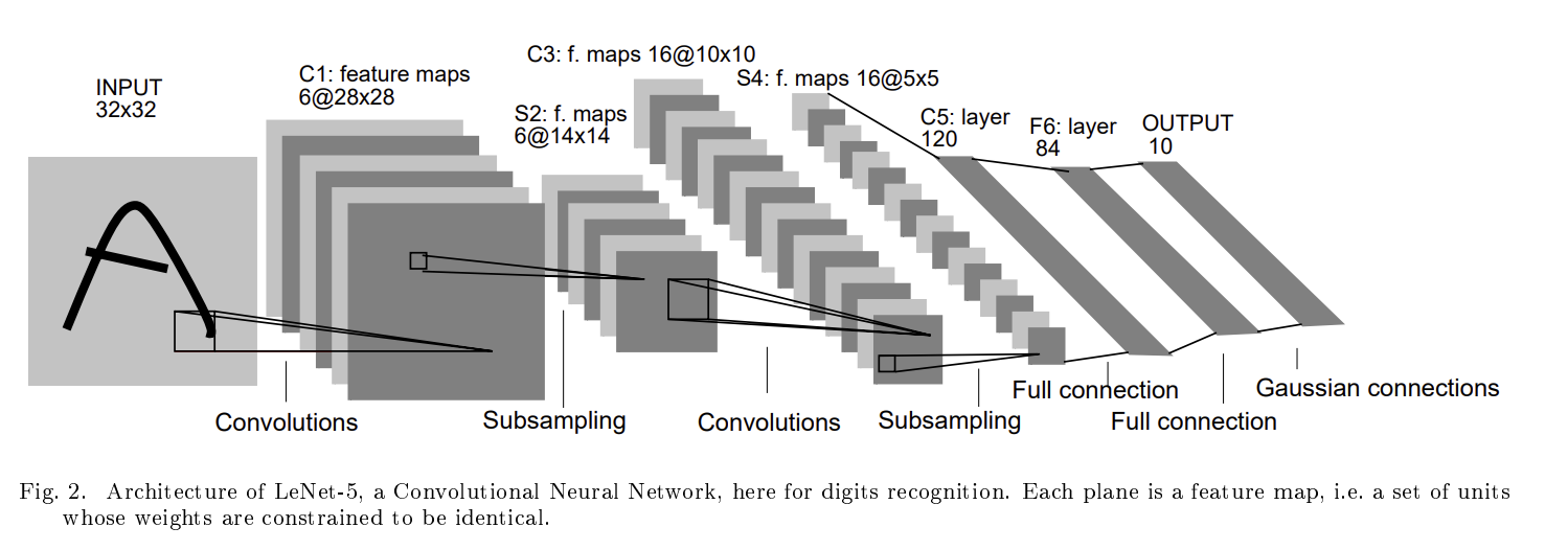
The figure above shows the neural network architecture diagram from the original paper, where:

• INPUT — input layer, a 32x32 grayscale image
• C1 Convolutions — convolutional layer with 6 kernels of size 5x5, producing 6 feature maps of size 28x28
• S2 Subsampling — downsampling layer (now commonly called pooling): each feature map is downsampled to produce 6 feature maps of size 14x14
• C3 Convolutions — 16 kernels, producing 16 feature maps of size 10x10
• S4 — downsampling layer (pooling), producing 16 feature maps of size 5x5
• C5 Full Connection — fully connected convolutional layer: although it still uses convolution kernels, because the input is only 5x5, the kernel covers the entire region, effectively functioning as a fully connected layer (120 nodes)
• F6 — fully connected layer with 84 nodes
• OUTPUT — output layer with 10 units, corresponding to the digit classes 0–9

The detailed meaning of each component will be covered gradually in later sections. Nowadays, LeCun's diagram is typically drawn as follows:

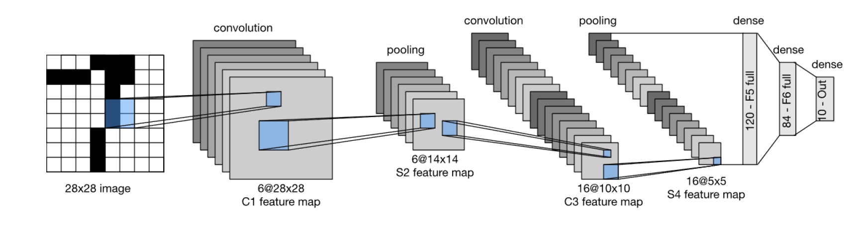
The main differences between the modern and original versions are:

• The input is drawn as 28x28, omitting the zero-padding step
• The output is labeled directly as dense/output10, no longer emphasizing Gaussian connections, since modern implementations almost universally use softmax
• Modern convention favors labeling layers as convolution / pooling / dense

Convolution (convolutional layer) extracts local features from the input image by sliding a small filter (kernel) across the image, computing a weighted sum over each local region to produce a feature map. Its purpose is to detect patterns such as edges, corners, and curves.

Pooling (pooling / downsampling layer) reduces the spatial dimensions of the feature map while preserving the most important information, thereby reducing computational cost. Common methods include:

• Average Pooling: takes the regional average
• Max Pooling: takes the regional maximum (more common in modern networks)

The S2 layer in LeNet-5 (reducing 28x28 to 14x14) and the S4 layer (reducing 10x10 to 5x5) both use average pooling.

Dense (fully connected layer) integrates all previously extracted features and maps them to the final classification or regression output. Each neuron is connected to every neuron in the preceding layer, performing a weighted sum before passing the result to the next layer. In LeNet-5, F5 has 120 neurons, F6 has 84 neurons, and the output layer has 10 neurons (corresponding to the 10 digit classes).

---

With these basic concepts in hand, we can now use LeNet-5 to run an MNIST experiment. At this stage, we do not need to master every detail (I am also just beginning to learn deep learning myself). The goal of this experiment is simply to gain an overall impression of the content and workflow of neural network training. Personally, I also took this opportunity to practice using my university's HPC resources — after all, tuition has already been paid, so I might as well make good use of them instead of spending my own money on compute or wearing out my personal machine.

The relevant experiment files are as follows:

• mnist.py: Data preparation — downloading, loading, and preprocessing the MNIST dataset (corresponds to the first notebook cell)
• lenet5.py: Model architecture definition — implementing the LeNet-5 CNN (corresponds to the second notebook cell)
• lenet5_train.py: Training the LeNet-5 model (corresponds to the third notebook cell) and plotting training curves (corresponds to the fifth notebook cell)
• checkpoint.py: Utilities for saving and resuming training from checkpoints (corresponds to the fourth notebook cell)

(1) mnist.py

import torch # torch is the main PyTorch library
from torchvision import datasets, transforms
# torchvision is PyTorch's official computer vision toolkit
# torchvision.datasets provides common vision datasets
# torchvision.transforms provides image preprocessing utilities
# torchvision.models provides pretrained models
#   torchvision offers many classic CNN architectures and pretrained models, such as:
#       AlexNet, VGG, ResNet, DenseNet, MobileNet, EfficientNet
#       These pretrained models can be loaded directly for transfer learning
from torch.utils.data import random_split, DataLoader
# random_split is used to split training and validation sets
# DataLoader wraps data into iterable mini-batches for training loops

DATASET_DIR = "datasets/downloads"
# Directory for storing the dataset; if not present locally, PyTorch will automatically download it here

def get_loaders(batch_size: int = 128, val_fraction: float = 0.2):
    """
    INPUT: MNIST data pipeline
    RETURN: Three iterators:
                        train_loader for training
                        val_loader for validation
                        test_loader for testing
    Parameters:
            batch_size: number of samples per mini-batch (default 128)
            val_fraction: fraction of the training set reserved for validation (default 20%)
    """
    # Preprocessing: convert images to tensors
    # Scalar: a 0-dimensional tensor, e.g., 3.14
    # Vector: a 1-dimensional tensor, e.g., [1, 2, 3]
    # Matrix: a 2-dimensional tensor
    #       Original MNIST pixel values range from 0–255 (uint8).
    #       transforms.ToTensor() converts them to floating-point tensors in [0, 1]:
    #                Black pixel = 0
    #                White pixel = 1
    #                Gray pixel = a decimal between 0 and 1
    #
    # After conversion, each pixel value (e.g., 0.5) is a 0D tensor
    # A single MNIST image is 28x28 pixels; as a tensor it is a 2D tensor of shape [28, 28]
    # Since MNIST is grayscale, there is also a channel dimension, making it a 3D tensor of shape [1, 28, 28]
    #
    # After batching with DataLoader (e.g., batch size = 128),
    # one batch becomes a 4D tensor, e.g., [128, 1, 28, 28]
    transform = transforms.ToTensor()

    # Download dataset and specify split
    full_train = datasets.MNIST(DATASET_DIR, train=True, download=True, transform=transform)
    test_ds    = datasets.MNIST(DATASET_DIR, train=False, download=False, transform=transform)

    # Use the given val_fraction to define train_size and val_size
    # Train/validation split (reproducible random split with seed 42)
    train_size = int((1 - val_fraction) * len(full_train))
    val_size   = len(full_train) - train_size
    generator  = torch.Generator().manual_seed(42)
    train_ds, val_ds = random_split(full_train, [train_size, val_size], generator=generator)

    # Wrap the datasets with DataLoader, similar to train_loader
    # Wrap into DataLoaders for batching, shuffling, and parallel loading
    train_loader = DataLoader(train_ds, batch_size=batch_size, shuffle=True)
    val_loader   = DataLoader(val_ds,   batch_size=batch_size, shuffle=False)
    test_loader  = DataLoader(test_ds,  batch_size=batch_size, shuffle=False)

    return train_loader, val_loader, test_loader

(2) lenet5.py

import torch
import torch.nn as nn
# torch.nn: neural network module containing various layers — convolution, linear, pooling, etc.
# torch.nn.functional: provides lower-level functional interfaces
import torch.nn.functional as F

class LeNet5(nn.Module):
    """
    Model class definition and network structure initialization.
    LeNet-5 for MNIST (28x28, 1 channel).
    C1: 1 -> 6 (5x5) -> 28x28
    S2  -> 6@14x14
    C3: 6 -> 16 (5x5) -> 10x10
    S4: -> 16@5x5
    F5: 16@5x5 -> 120
    F6: 120 -> 84
    Out: 84 ->10
    """
    def __init__(self):
        super().__init__()

        # Feature extraction
        self.net = nn.Sequential(
            nn.Conv2d(in_channels=1, out_channels=6, kernel_size=5, stride=1, padding=2),   # 28*28->32*32-->28*28
            nn.Tanh(),
            nn.AvgPool2d(kernel_size=2, stride=2),  # 14*14
            nn.Conv2d(in_channels=6, out_channels=16, kernel_size=5, stride=1),  # 10*10
            nn.Tanh(),
            nn.AvgPool2d(kernel_size=2, stride=2),  # 5*5
        )

        # Classification head
        self.classifier = nn.Sequential(
            nn.Flatten(),
            nn.Linear(in_features=16*5*5, out_features=120),
            nn.Tanh(),
            nn.Linear(in_features=120, out_features=84),
            nn.Tanh(),
            nn.Linear(in_features=84, out_features=10),
        )

    def forward(self, x):
        """
        Forward pass:
            Input x has shape [batch, 1, 28, 28].
            First passes through convolution + pooling for feature extraction (self.net).
            Then passes through fully connected layers for classification (self.classifier).
            Output shape is [batch, 10], with each sample producing 10 class logits.
        """
        return self.classifier(self.net(x))

(3) lenet5_train.py

import torch
import torch.nn as nn
import matplotlib.pyplot as plt
import os
import time

from mnist import get_loaders
from lenet5 import LeNet5
from checkpoint import Checkpointer

def train_one_epoch(model, loader, criterion, optimizer, device):
    """
    Train `model` for a single epoch.

    Args:
        model:    the neural network being trained
        loader:    DataLoader that yields (inputs, labels) mini-batches
        criterion:  l
        s function (e.g., CrossEntropyLoss)
        optimizer:  optimizer instance (e.g., SGD/Adam)
        device:    torch.device("cuda") for GPUs or torch.device("cpu") for CPUs

    Returns:
        avg_loss:   average training loss over all samples in this epoch
        acc:    training accuracy (%) over all samples in this epoch
    """
    model.train() # enable training mode
    running_loss = 0.0
    correct = total = 0
    for x, y in loader:
        # Move the mini-batch to the target device (GPU/CPU)
        x, y = x.to(device), y.to(device)
        # 1) Important!!!: Clear gradients from the previous optimization step
        optimizer.zero_grad()
        # 2) Forward pass: compute logits/predictions
        pred = model(x)
        # 3) Compute loss between predictions and the true labels
        loss = criterion(pred, y)
        # 4) Backward propagation: compute gradients w.r.t. model parameters
        loss.backward()
        # 5) Update model parameters (weight, bias)
        optimizer.step()

        # Accumulate loss (sum over samples) for epoch-level averaging
        running_loss += loss.item() * x.size(0)
        # Convert logits to predicted class indices and count correct predictions
        preds = pred.argmax(dim=1)
        correct += (preds == y).sum().item()
        total += y.size(0)

    return running_loss / total, 100 * correct / total


def eval_one_epoch(model, loader, criterion, device):
    """
    Evaluate `model` for a single epoch on the validation/test dataset.

    Args:
        model:    the neural network being trained
        loader:    DataLoader that yields (inputs, labels) mini-batches
        criterion:  loss function (e.g., CrossEntropyLoss)
        device:    torch.device("cuda") for GPUs or torch.device("cpu") for CPUs

    Returns:
        avg_loss:   average eval loss over all samples
        acc:    eval accuracy (%) over all samples in this epoch

    Notes:
        - We wrap the loop with `torch.no_grad()` so no gradients are tracked:
          * no backward pass, no optimizer steps
    """
    model.eval() # enable eval mode
    running_loss = 0.0
    correct = total = 0
    # Disable autograd during evaluation (no grad tracking / no backward)
    with torch.no_grad():
        for x, y in loader:
            x, y = x.to(device), y.to(device)
            pred = model(x) # Forward pass only
            loss = criterion(pred, y)

            running_loss += loss.item() * x.size(0)
            preds = pred.argmax(dim=1)
            correct += (preds == y).sum().item()
            total += y.size(0)

    return running_loss / total, 100 * correct / total

#===================================================================================================================================
# ADD YOUR CODES HERE
# Plot and save curves for train/val loss/accuracy.
# def plot_results():
import csv

def _ensure_dir(path: str):
    os.makedirs(path, exist_ok=True)


def save_history_csv(hist, outdir="plots", run_name="run"):
    _ensure_dir(outdir)
    csv_path = os.path.join(outdir, f"{run_name}_history.csv")
    epochs = len(hist["train_loss"])
    with open(csv_path, "w", newline="") as f:
        w = csv.writer(f)
        w.writerow(["epoch", "train_loss", "train_acc", "val_loss", "val_acc", "epoch_time"])
        for e in range(epochs):
            w.writerow([
                e + 1,
                hist["train_loss"][e],
                hist["train_acc"][e],
                hist["val_loss"][e],
                hist["val_acc"][e],
                hist["epoch_time"][e] if e < len(hist["epoch_time"]) else 0.0
            ])
    return csv_path


def plot_results_single(hist, outdir="plots", run_name="run"):
    _ensure_dir(outdir)
    epochs = list(range(1, len(hist["train_loss"]) + 1))

    plt.figure()
    plt.plot(epochs, hist["train_loss"], label="train loss")
    plt.xlabel("Epoch")
    plt.ylabel("Loss")
    plt.title(f"Training Loss ({run_name})")
    plt.grid(True)
    plt.legend()
    plt.savefig(os.path.join(outdir, f"{run_name}_train_loss.png"), bbox_inches="tight")
    plt.close()

    plt.figure()
    plt.plot(epochs, hist["train_acc"], label="train acc")
    plt.xlabel("Epoch")
    plt.ylabel("Accuracy (%)")
    plt.title(f"Training Accuracy ({run_name})")
    plt.grid(True)
    plt.legend()
    plt.savefig(os.path.join(outdir, f"{run_name}_train_acc.png"), bbox_inches="tight")
    plt.close()

    plt.figure()
    plt.plot(epochs, hist["val_loss"], label="val loss")
    plt.xlabel("Epoch")
    plt.ylabel("Loss")
    plt.title(f"Validation Loss ({run_name})")
    plt.grid(True)
    plt.legend()
    plt.savefig(os.path.join(outdir, f"{run_name}_val_loss.png"), bbox_inches="tight")
    plt.close()

    plt.figure()
    plt.plot(epochs, hist["val_acc"], label="val acc")
    plt.xlabel("Epoch")
    plt.ylabel("Accuracy (%)")
    plt.title(f"Validation Accuracy ({run_name})")
    plt.grid(True)
    plt.legend()
    plt.savefig(os.path.join(outdir, f"{run_name}_val_acc.png"), bbox_inches="tight")
    plt.close()


def plot_results_multi(all_histories, all_labels, outdir="plots"):
    _ensure_dir(outdir)
    metrics = [
        ("train_loss", "Training Loss", "Loss"),
        ("train_acc", "Training Accuracy", "Accuracy (%)"),
        ("val_loss", "Validation Loss", "Loss"),
        ("val_acc", "Validation Accuracy", "Accuracy (%)"),
    ]

    for key, title, ylabel in metrics:
        plt.figure()
        for hist, label in zip(all_histories, all_labels):
            epochs = list(range(1, len(hist[key]) + 1))
            plt.plot(epochs, hist[key], label=label)
        plt.xlabel("Epoch")
        plt.ylabel(ylabel)
        plt.title(title)
        plt.grid(True)
        plt.legend()
        plt.savefig(os.path.join(outdir, f"{key}.png"), bbox_inches="tight")
        plt.close()


def main(ckpt, device, seed, lr, epochs, batch_size, run_name=None):
    if run_name is None:
        run_name = f"lenet5_lr{lr}_bs{batch_size}"

    train_loader, val_loader, test_loader = get_loaders(batch_size=batch_size)

    torch.manual_seed(seed)
    if torch.cuda.is_available():
        torch.cuda.manual_seed_all(seed)

    model = LeNet5().to(device)
    criterion = nn.CrossEntropyLoss()
    optimizer = torch.optim.SGD(model.parameters(), lr=lr)

    hist = {"train_loss": [], "train_acc": [], "val_loss": [], "val_acc": [], "epoch_time": []}

    start_epoch = 0
    try:
        out = ckpt.resume(model, optimizer, hist)
        if isinstance(out, tuple) and len(out) == 2:
            start_epoch, hist = out
        elif isinstance(out, int):
            start_epoch = out
        else:
            start_epoch = 0
    except (FileNotFoundError, IOError, AttributeError):
        start_epoch = 0

    for epoch in range(start_epoch + 1, epochs + 1):
        t0 = time.perf_counter()

        tr_loss, tr_acc = train_one_epoch(model, train_loader, criterion, optimizer, device)
        va_loss, va_acc = eval_one_epoch(model, val_loader, criterion, device)

        elapsed = time.perf_counter() - t0

        hist["train_loss"].append(tr_loss)
        hist["train_acc"].append(tr_acc)
        hist["val_loss"].append(va_loss)
        hist["val_acc"].append(va_acc)
        hist["epoch_time"].append(elapsed)

        print(f"[{run_name}] Epoch {epoch}/{epochs} | "
              f"Train: loss={tr_loss:.4f}, acc={tr_acc:.2f}% | "
              f"Val: loss={va_loss:.4f}, acc={va_acc:.2f}% | "
              f"time: {elapsed:.2f}s")

        try:
            ckpt.save(epoch, model, optimizer, hist,
                      config={"lr": lr, "batch_size": batch_size, "run_name": run_name})
        except Exception as e:
            print(f"[{run_name}] Warning: checkpoint save failed: {e}")

    t1 = time.perf_counter()
    te_loss, te_acc = eval_one_epoch(model, test_loader, criterion, device)
    elapsed1 = time.perf_counter() - t1
    print(f"[{run_name}] Test: loss={te_loss:.4f}, acc={te_acc:.2f}% | time: {elapsed1:.2f}s")

    plot_results_single(hist, outdir="plots", run_name=run_name)
    save_history_csv(hist, outdir="plots", run_name=run_name)

    return hist


if __name__ == "__main__":
    device = torch.device("cuda" if torch.cuda.is_available() else "cpu")
    print(f"Using device: {device}")

    learning_rates = [1e-1, 1e-2, 1e-3]
    batch_sizes = [64, 128]
    epochs = 100
    seed = 42

    all_histories = []
    all_labels = []

    for lr in learning_rates:
        for bs in batch_sizes:
            run_name = f"lenet5_lr{lr}_bs{bs}"
            ckpt_dir = os.path.join("checkpoints", run_name)
            os.makedirs(ckpt_dir, exist_ok=True)

            ckpt_path = os.path.join(ckpt_dir, "ckpt.pth")
            ckpt = Checkpointer(path=ckpt_path, device=device)

            hist = main(
                ckpt=ckpt,
                device=device,
                seed=seed,
                lr=lr,
                epochs=epochs,
                batch_size=bs,
                run_name=run_name
            )

            all_histories.append(hist)
            all_labels.append(f"lr={lr}, bs={bs}")

    plot_results_multi(all_histories, all_labels, outdir="plots")

(4) checkpoint.py

import os, torch
from pathlib import Path
from dataclasses import dataclass

@dataclass
class Checkpointer:
    path: str
    device: torch.device

    def save(self, epoch: int, model, optimizer=None, hist=None, config=None):
        """
        Atomically save a checkpoint to `path`.
        This reduces the risk of a half-written file if the job is killed mid-save.
        """
        payload = {
            "epoch": epoch,
            "model_state_dict": model.state_dict(),
            "cpu_rng_state": torch.get_rng_state(),
        }
        if torch.cuda.is_available():
            payload["cuda_rng_state_all"] = torch.cuda.get_rng_state_all()
        if optimizer is not None:
            payload["optimizer_state_dict"] = optimizer.state_dict()
        if hist is not None:
            payload["hist"] = hist
        if config is not None:
            payload["config"] = config

        tmp = self.path + ".tmp"
        torch.save(payload, tmp)
        os.replace(tmp, self.path)

    def resume(self, model, optimizer=None, hist=None):
        """
        Resume training state from `ckpt_path` if it exists.

        Restores:
          - model parameters
          - optimizer state (if provided)
          - RNG states (CPU + all CUDA devices, if available)
          - last finished epoch
          - training/validation history

        Returns:
          start_epoch (int): last finished epoch number (0 if none)
          hist      (dict): metric history dict with lists
        """
        p = Path(self.path)
        start_epoch = 0
        hist = hist or {"train_loss": [], "train_acc": [], "val_loss": [], "val_acc": [], "epoch_time": [] }
        if not p.exists():
            print(f"[resume] No checkpoint at {p}; starting from scratch.")
            print("-------------------------------------------------------------------")
            return start_epoch, hist

        ckpt = torch.load(p, map_location="cpu", weights_only=False)
        model.load_state_dict(ckpt["model_state_dict"])
        if optimizer is not None and "optimizer_state_dict" in ckpt:
            optimizer.load_state_dict(ckpt["optimizer_state_dict"])
        if "cpu_rng_state" in ckpt:
            torch.set_rng_state(ckpt["cpu_rng_state"])
        if torch.cuda.is_available() and "cuda_rng_state_all" in ckpt:
            torch.cuda.set_rng_state_all(ckpt["cuda_rng_state_all"])
        start_epoch = ckpt.get("epoch", 0)
        if "hist" in ckpt and ckpt["hist"] is not None:
            hist = ckpt["hist"]

        print(f"[resume] Loaded {p}: last finished epoch = {start_epoch}")
        print("-------------------------------------------------------------------")
        return start_epoch, hist

    def remove(self):
        """
        Delete checkpoint file if it exists (fresh start).
        """
        p = Path(self.path)
        if p.exists():
            p.unlink()
            print(f"Removed checkpoint: {p.resolve()}")
        else:
            print(f"No checkpoint found at: {p.resolve()}")

After training, we obtain the following four plots:

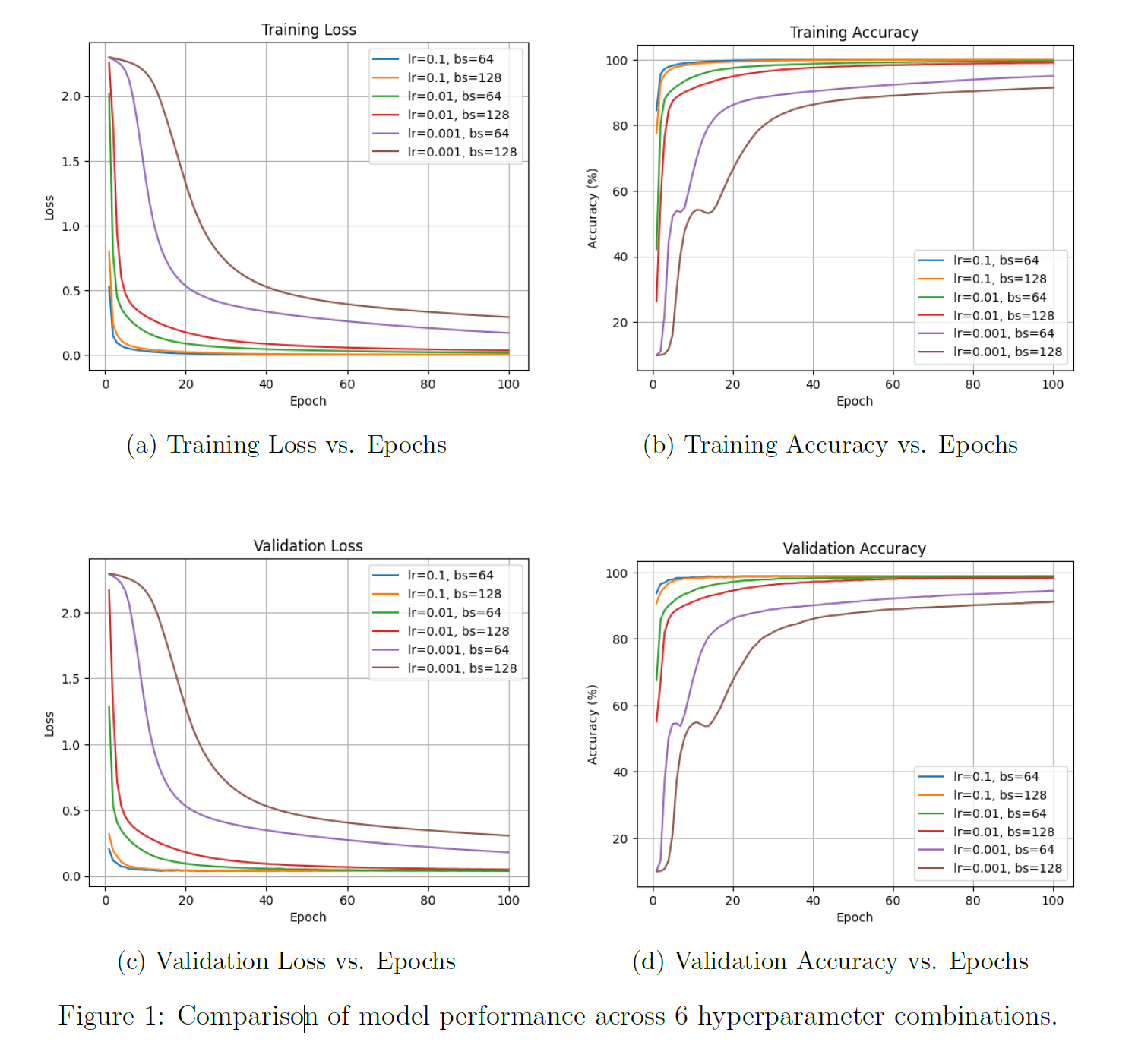
In brief, the overall experimental workflow is as follows:

1. Task definition: Train the classic LeNet-5 convolutional neural network architecture on the MNIST dataset, which contains 60,000 training images, for a classification task.
2. Experiment design: Design a grid search experiment with 6 different hyperparameter combinations, varying learning rate (0.1, 0.01, 0.001) and batch size (64, 128).
3. Execution and evaluation: Run each of the 6 experimental configurations for 100 epochs. After each epoch, record the model's accuracy and loss on both the training and validation sets to monitor model performance.

From the four result plots, the impact of different hyperparameter combinations on the training process and final performance is clearly visible. For example, we can observe:

Learning rate is the decisive factor:

• With a learning rate of 0.1 (blue and orange curves), the model performs best. It converges the fastest and achieves a peak validation accuracy of approximately 99%.
• With a learning rate of 0.01 (green and red curves), the model performs well, but convergence speed and final performance are slightly inferior.
• With a learning rate of 0.001 (purple and brown curves), the model performs poorly. The excessively low learning rate causes extremely slow convergence, and after 100 epochs of training, the model is far from optimal.

Batch size has a smaller impact:

• At effective learning rates (0.1 and 0.01), the curves for batch size 128 are somewhat smoother than those for 64, but the final performance is nearly identical.

In summary, through the above experiments, we successfully verified that the classic LeNet-5 architecture can achieve very high recognition accuracy on the MNIST task when appropriate hyperparameters are selected. This example serves as an introductory case study, helping us understand what a neural network architecture is, how to translate such an architecture into Python code, how to use PyTorch for training and evaluation, and how to design experiments and test architectures. In subsequent chapters, we will discuss more complex architectures and more sophisticated experiments, but the core methodology will not differ substantially from the process described above. That is, a typical experiment generally involves the following steps:

1. Define the problem — determine whether the task is image classification, object detection, or something else.
2. Prepare and preprocess the data, then split it into training, validation, and test sets. The validation set is crucial for hyperparameter tuning; the test set is reserved for final evaluation.
3. Choose an architecture: Based on the task complexity and data characteristics, select an appropriate neural network architecture such as LeNet-5, ResNet, Transformer, etc.
4. Implement the chosen architecture using a mature deep learning framework like PyTorch or TensorFlow, defining each layer and the forward propagation path in code.
5. Define the training pipeline, including the loss function, optimizer, and training loop.
6. Design experiments to systematically search for the best hyperparameter combination (e.g., learning rate, batch size, network depth). Grid search is commonly used.
7. Execute training. Small-scale tasks can be completed on a personal computer, while large-scale tasks require HPC cluster resources. Use a checkpoint mechanism to save progress. Throughout training, continuously monitor performance on the validation set to determine whether the model is improving, whether overfitting is occurring, and ultimately select the model that performs best on the validation set.
8. Finally, analyze the results and draw conclusions. Typically, various metrics from the training process — such as loss and accuracy curves — are visualized. Then, result plots from different experiments are compared to analyze how hyperparameters affect model performance, identify the optimal configuration, and explain the underlying reasons. Remember to perform a generalization test — evaluate on a test set the model has never seen, or on real-world cases that differ significantly from the test set — to produce a final, objective performance report.

CIFAR-10 and Optimizer Comparison

In the introductory chapter, we conducted a LeNet-5 experiment on the MNIST handwritten digit dataset and learned the basics of the deep learning training process. After studying optimizers, we now conduct a new experiment to test the training performance of different optimizers on the CIFAR-10 dataset.

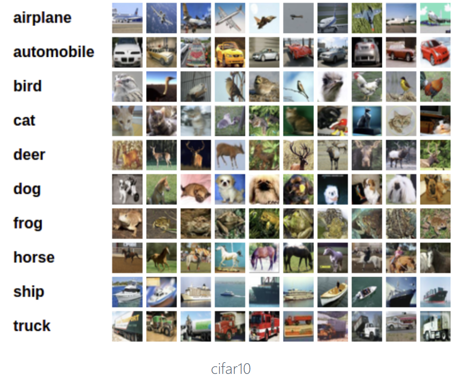
Compared to MNIST, CIFAR-10 does not increase the number of classes — there are still 10 categories — but the complexity of the objects to be recognized is significantly greater: the images are 32x32-pixel RGB three-channel color images with cluttered backgrounds and low resolution.

We use the following three architectures to experiment on MNIST and CIFAR-10:

• A simple MLP on MNIST
• A simple CNN on CIFAR-10
• VGG-13 on CIFAR-10

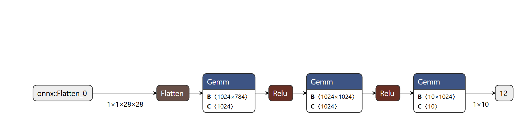
Simple MLP (for the MNIST task):

• Input: a single 1x28x28 image, where 1 represents one channel (grayscale)
• Flatten converts the 2D image into a 1x784 one-dimensional vector (i.e., all pixels in the image grid are arranged into a single sequence)
• Then it passes through the first hidden layer (Gemm): this is the first fully connected layer of the network, which takes the 784-length input vector and, through a 1024x784 weight matrix B, linearly transforms it into a 1024-length hidden feature vector — this is where the network begins learning abstract features from raw pixels
• ReLU: the activation function that follows, adding nonlinearity so the network can learn more complex relationships
• Then comes the second hidden layer
• Finally, it connects to the last Gemm — the output layer, which maps the 1024-dimensional high-level features from the second hidden layer to 10 output values

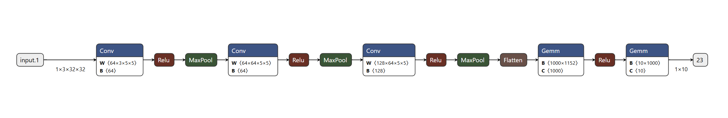
Three-layer CNN (for the CIFAR task):

• Input: a single RGB color 3-channel 32x32-pixel image
• Data flows left to right through three identical processing blocks: Conv (convolutional layer) -> ReLU (activation layer) -> MaxPool (max pooling layer)
• Flatten layer
• Gemm (fully connected layer)
• Final output: a 1x10 vector corresponding to the probability of each of the 10 classes; the highest score is the predicted class

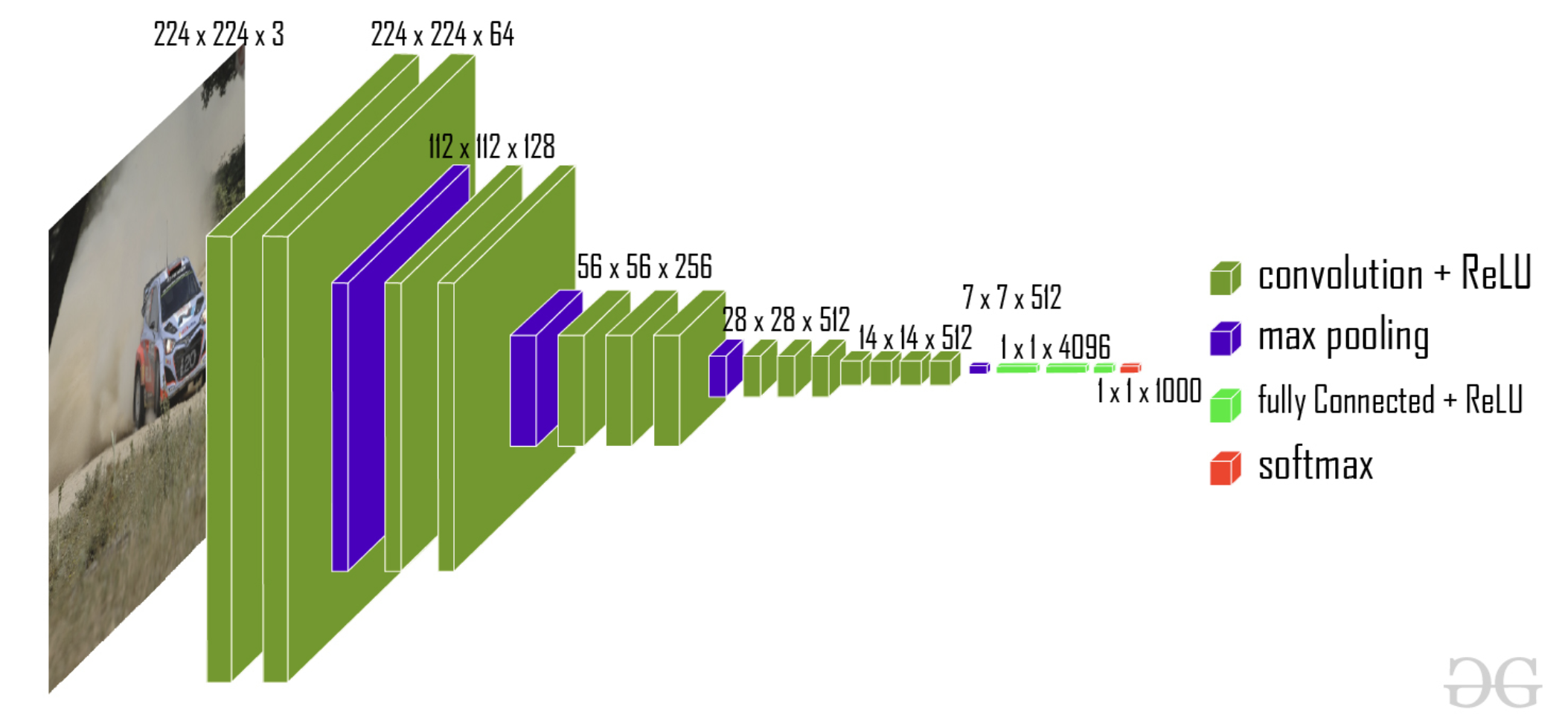
VGG-13 (for the CIFAR task):

• The figure below shows VGG-16; in our experiment we use VGG-13 from the same family, simplified for CIFAR. VGG was invented by the Visual Geometry Group at Oxford University and is named accordingly. VGG-13 has 10 convolutional layers + 3 fully connected layers; VGG-16 has 13 convolutional layers + 3 fully connected layers.
• VGG-13/VGG-16 enforces a strict design choice for kernel size: all convolutional kernels are uniformly 3x3.

Training code is available in the repository:

Project report available at:

Results are as follows:

Optimizer	MLP on MNIST	CNN on CIFAR-10	VGG13 on CIFAR-10
SGD	91.82%	50.64%	52.68%
AdaGrad	97.77%	69.98%	68.11%
RMSProp	98.29%	68.65%	73.61%
Adam	98.32%	70.15%	74.61%
Polyak_0.9	97.64%	73.00%	65.75%
Nesterov_0.9	97.62%	72.91%	66.02%

Overall, Adam delivers the best performance, while Polyak and Nesterov momentum methods outperform Adam on the CNN on CIFAR-10 task.

---

ImageNet-50 with Different Initialization and Learning Rate Scheduler Experiments

Dataset and DNN

ImageNet-50 (Customized)

ImageNet is a relatively small subset of the ImageNet dataset for image classification tasks. The original ImageNet contains over 14 million images spanning approximately 22,000 categories and has been a pivotal dataset driving the development of deep learning in computer vision.

This project selected 50 target classes from ImageNet (sourced from ILSVRC-2012). During preprocessing, each image was converted to RGB format and resized to 224 x 224 to ensure input consistency. Each class contains approximately 1,300 images, covering a rich variety of animals, plants, and other familiar everyday objects.

VGG-19

VGG-19 is a convolutional neural network architecture from the VGG (Visual Geometry Group) family, renowned for its small kernel size (3x3) and deep structure.

This project deployed a modified version of VGG-19 (improved by He et al.), which, compared to the original VGG-19, adopts larger convolutional layers in the early stages and increases the model's depth to improve efficiency and performance on the ImageNet training set.

ResNet-34

ResNet-34 is a specific version of the Residual Network (ResNet) architecture, where 34 denotes the total number of learnable weight layers (including convolutional and fully connected layers) in this particular network.

Residual learning introduces the concept of residual blocks, sometimes also called skip connections. Each residual block contains two 3x3 convolutional layers followed by batch normalization and ReLU activation. Residual blocks allow information to bypass certain layers and propagate directly, thereby alleviating the problems of vanishing gradients and network degradation in deep neural networks. This enables the construction of very deep networks while maintaining effective training.

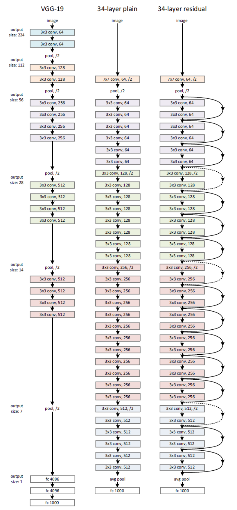
The figure above compares three DNN architectures:

Left	Middle	Right
VGG-19	Plain 34-layer	ResNet-34
CNN	CNN	CNN
No residual connections	No residual connections	With residual connections

.

Project Objectives and Result Analysis

This project investigates how weight initialization methods and learning rate schedulers affect DNN model training.

Weight initialization determines how a model's parameters are set before training begins, affecting the model's:

• Ability to converge
• Convergence speed
• Stability

Learning rate schedulers determine the step size of gradient updates, influencing how the cost function adapts to training steps and convergence performance.

Learning rate schedulers critically affect:

• Training results: loss function
• Test results: test accuracy

Weight Initialization on VGG-19

Setting appropriate initial values in DNN training is a major challenge. Improper initialization can lead to gradient explosion, vanishing gradients, slow convergence, and degraded accuracy.

The objective of this experiment is to compare the following two initialization strategies on VGG-19:

• Xavier Initialization
• Kaiming Initialization

as well as the following two distributions:

• Uniform Distribution
• Normal Distribution

In this experiment, we use the SGD optimizer to isolate the effects of different initializations.

The experiment therefore consists of four controlled groups:

• Xavier Initialization + Uniform Distribution
• Xavier Initialization + Normal Distribution
• Kaiming Initialization + Uniform Distribution
• Kaiming Initialization + Normal Distribution

The outputs include:

• Training loss vs. epochs
• Training accuracy vs. epochs
• Validation loss vs. epochs
• Validation accuracy vs. epochs
• Final test accuracy and test loss

LR Scheduling on ResNet-34

Another major challenge in DNN training is setting an appropriate learning rate schedule. Improper settings can lead to training instability, excessively slow convergence, or convergence to local optima.

In this experiment, we use the ResNet model to explore the effects of different learning rate schedules on training:

(1) Constant Learning Rate

A constant learning rate means the learning rate remains unchanged throughout the entire training process (no scheduling or adjustment is applied). This is the simplest baseline method.

(2) Exponential Learning Rate

Gradually reducing the LR from max to min according to some fixed schedule.

The exponential learning rate is a specific method that decays the learning rate according to an exponential function or geometric progression.

(3) Multistep Learning Rate

The multistep learning rate is another form of fixed scheduling, where the learning rate drops by a fixed factor at predetermined epoch milestones (e.g., reduced to 0.1x every 30 epochs).

(4) Cyclic Learning Rate

Having multiple cycles of LR reduction from max to min.

The cyclic learning rate varies the learning rate periodically between predefined bounds (a maximum and minimum), typically following a triangular or sinusoidal waveform.

(5) Cosine Annealing Warm Restarts

Cosine annealing with warm restarts also cycles the learning rate from max to min, following the shape of a cosine function for decay. When the learning rate reaches its minimum, it "warm restarts" by jumping back to the maximum value and begins cosine decay again.

For ResNet-34, we use the Adam optimizer. Weight initialization uses Kaiming Uniform Distribution (which is also PyTorch's default initialization method).

---

Below are the specific parameter settings for the four non-constant learning rate schedulers:

Exponential (Exponential Decay):

• Parameter setting: \(\text{Gamma} = 0.95\).
• Mechanism: The learning rate is multiplied by the decay factor \(0.95\) at the end of each epoch (or step), achieving a smooth decrease.

Multistep (Multistep Decay):

• Parameter setting: \(\text{Milestones} = [40, 60, 80]\) and \(\text{Gamma} = 0.1\).
• Mechanism: The learning rate drops sharply at the predetermined epochs \(40\), \(60\), and \(80\).
• At each milestone, the current learning rate is multiplied by \(0.1\).

Cyclic (Cyclic Learning Rate):

• Parameter setting: \(\text{base\_lr} = 5\text{e-}4\) (\(\text{minimum learning rate}\)), \(\text{max\_lr} = 5\text{e-}3\) (\(\text{maximum learning rate}\)), \(\text{step\_size\_up} = 2380\), and \(\text{mode} = \text{'triangular'}\).
• Mechanism: The learning rate cycles periodically between \(0.0005\) and \(0.005\).
• One complete half-cycle (ascending or descending) takes \(2380\) steps (iterations).
• The waveform uses the basic triangular mode.

Cosine Annealing Warm Restarts:

• Parameter setting: \(\text{T\_0} = 10\) and \(\text{T\_mult} = 3\).
• Mechanism: The learning rate decays following a cosine function and periodically restarts.
• The initial cycle length (\(\text{T\_0}\)) is \(10\) epochs.
• The cycle multiplication factor (\(\text{T\_mult}\)) is \(3\). After each warm restart, the duration of the next decay cycle is \(3\) times that of the previous one.

---

评论