Vision Transformer (ViT)
This note provides a systematic introduction to the Vision Transformer (ViT), covering its architecture, forward propagation process, major variants, and comparisons with CNNs. ViT was the first architecture to demonstrate that a pure Transformer can be directly applied to image classification, marking a turning point in computer vision from CNN dominance to Transformer dominance.
Background and Motivation
Visual Encoders
In deep learning, an encoder refers to any model that transforms raw data (such as pixels, audio, or words) into abstract feature vectors (embeddings). A visual encoder is a structure that takes an image as input and outputs a vector.
For the 20 years before the Transformer was introduced, CNNs were the undisputed champion of visual encoders. When we feed an image into a CNN-based neural network such as ResNet, it passes through the network, extracting features layer by layer, and ultimately outputs a feature vector. This entire process is "encoding."
After Transformers gained popularity, the concepts of Encoder (responsible for understanding input) and Decoder (responsible for generating output) became widely known. Before that, we rarely referred to CNNs as visual encoders — instead, they were called backbones or feature extractors. Around 2015, during the era of Image Captioning, researchers began connecting CNNs to RNNs. It was at this point that people started calling CNNs "Visual Encoders" and RNNs "Decoders."
Why Apply Transformers to Vision
CNNs have two inherent limitations:
- Limited receptive field: CNNs are inherently biased toward local modeling, making long-range dependency modeling difficult. Expanding the receptive field requires stacking more layers.
- Overly strong inductive bias: The two core assumptions of CNNs — translation invariance and local continuity — are too rigid, preventing the model from learning structure on its own.
After the Transformer architecture emerged, the Self-Attention mechanism replaced convolution and recurrence, providing global modeling and parallel computation capabilities.
The Attention mechanism has three key properties:
- Data-driven structure
- Weaker inductive bias
- Native global information modeling
Transformers were initially used for NLP tasks. As the technology matured, the convolution-free Vision Transformer was proposed in 2020, commonly abbreviated as ViT.
Paper Information
"An Image is Worth 16x16 Words: Transformers for Image Recognition at Scale" Alexey Dosovitskiy et al., Google Brain, 2020 (ICLR 2021)
The significance of the ViT architecture lies in its demonstration that CNNs are not the only solution — vision can be handled with pure Attention. The key to ViT's success was data. With the emergence of large-scale datasets such as JFT-300M, the paradigm of large models + large data became the dominant trend, pre-training became mainstream, and ViT gradually rose to prominence.
It is worth noting that on small datasets, CNNs still outperform ViT. This is because CNNs have strong inductive biases, whereas ViT requires more data to learn spatial structure.
ViT demonstrated that visual backbones can be more general-purpose and more scalable (scaling data and models like in NLP), which inspired widespread interest in visual large model pre-training. However, due to the insufficient scale of classification-labeled data, closed category sets, and expensive transfer, this approach quickly hit a wall. Eventually, researchers came up with the idea of "using language as supervision" — CLIP. CLIP uses contrastive learning to align images and text into a shared space, enabling open-vocabulary and zero-shot transfer capabilities.
ViT Architecture in Detail
Core Idea
The core idea of ViT is remarkably simple: treat an image as a sequence of "words."
In NLP, the input to a Transformer is a sequence of tokens. ViT's approach is to divide the image into a number of fixed-size patches, where each patch serves as a "visual token," and then feed them directly into a standard Transformer Encoder. The entire process uses no convolutional operations whatsoever.
Complete Architecture Diagram
  输入图像 (H x W x C)
       |
       v
  +--------------------------+
  | Patch Partition          |
  | 切成 N = HW/P² 个       |
  | P x P 大小的 patch       |
  +--------------------------+
       |
       v  每个 patch 展平为 P²C 维向量
  +--------------------------+
  | Linear Projection        |
  | (P²C) --> (D)            |
  | 即 Patch Embedding       |
  +--------------------------+
       |
       v  得到 N 个 D 维 token
  +--------------------------+
  | Prepend [CLS] Token      |
  | 序列长度 N --> N+1        |
  +--------------------------+
       |
       v
  +--------------------------+
  | + Position Embedding     |
  | 可学习的 1D 位置编码      |
  | (N+1) 个 D 维向量        |
  +--------------------------+
       |
       v
  +--------------------------+      +---------------------------------+
  | Transformer Encoder x L  | ---> | 每层的结构 (Pre-Norm):          |
  |                          |      |   z' = z + MSA(LN(z))           |
  |   L 层堆叠               |      |   z'' = z' + FFN(LN(z'))        |
  +--------------------------+      +---------------------------------+
       |
       v  取 [CLS] token 的输出
  +--------------------------+
  | MLP Classification Head  |
  | D --> num_classes         |
  +--------------------------+
       |
       v
     分类结果
Patch Embedding in Detail
This is the most critical first step of ViT: converting a 2D image into a 1D token sequence.
Step 1: Patch Partition
Given an input image of size \(H \times W \times C\) (height \(\times\) width \(\times\) number of channels), choose a patch size of \(P \times P\). The image is uniformly divided into non-overlapping patches:
where \(N\) is the total number of patches, which also equals the final sequence length (excluding the [CLS] token).
Typical Configurations
For a \(224 \times 224\) image with \(P = 16\): \(N = 224^2 / 16^2 = 196\) patches. For a \(224 \times 224\) image with \(P = 14\): \(N = 224^2 / 14^2 = 256\) patches.
Step 2: Flatten
Each patch has an original size of \(P \times P \times C\), which is flattened into a one-dimensional vector:
For example, with \(P = 16\) and \(C = 3\) (RGB image), each flattened patch has a dimensionality of \(16^2 \times 3 = 768\).
Step 3: Linear Projection
The flattened vector is passed through a learnable linear projection layer, mapping it to the Transformer's hidden dimension \(D\) (i.e., \(d_{\text{model}}\)):
where \(\mathbf{E} \in \mathbb{R}^{(P^2 C) \times D}\) is the projection matrix and \(\mathbf{b} \in \mathbb{R}^{D}\) is the bias.
Implementation Trick
In practice, the three steps of Patch Partition + Flatten + Linear Projection are typically implemented efficiently using a convolution with stride equal to the patch size:
# PyTorch 实现
self.proj = nn.Conv2d(
    in_channels=C,           # 输入通道数 (如 3)
    out_channels=D,          # 输出维度 (如 768)
    kernel_size=P,           # 卷积核大小 = patch 大小
    stride=P                 # 步长 = patch 大小, 不重叠
)
# 输入: (B, C, H, W) --> 输出: (B, D, H/P, W/P)
# reshape 后: (B, N, D)  其中 N = (H/P) * (W/P)
[CLS] Token
Following the approach from BERT, ViT prepends a special learnable token to the beginning of the patch embedding sequence, called the [CLS] token (classification token).
where:
- \(\mathbf{x}_{\text{class}} \in \mathbb{R}^{D}\) is a learnable parameter vector, randomly initialized and updated during training
- The semicolons \(;\) denote concatenation along the sequence dimension
- After adding the [CLS] token, the sequence length changes from \(N\) to \(N + 1\)
Why is the [CLS] token needed?
The [CLS] token does not correspond to any specific image patch. Its role is to aggregate information from all patches through Self-Attention across multiple layers of the Transformer Encoder, ultimately serving as the global representation of the entire image. The classification head only needs to read the output of the [CLS] token to perform classification.
Alternative Approach
The original paper also experimented with not using a [CLS] token, instead applying Global Average Pooling (GAP) over all patch token outputs as the image representation. Experiments showed that both approaches performed comparably, but using the [CLS] token is more consistent with the NLP Transformer design convention. In some subsequent works (e.g., DeiT), GAP sometimes performs better.
Position Embedding
Self-Attention is inherently permutation invariant — it does not care about the order of tokens. However, for images, the spatial position of patches is clearly important: a patch in the upper-left corner and one in the lower-right corner carry different meanings. Therefore, positional information must be injected.
ViT uses learnable 1D Position Embeddings:
This is a learnable parameter matrix where each row corresponds to a position (including the [CLS] position), learned through backpropagation during training.
Difference from the Standard Transformer
The standard Transformer ("Attention Is All You Need") uses fixed sinusoidal positional encoding, whereas ViT uses learnable positional encoding. Experiments in the original paper showed that learnable 1D positional encoding performs comparably to hand-designed 2D positional encoding, indicating that the model can learn 2D spatial structure from 1D positional encoding on its own.
Why 1D instead of 2D?
Although image patches naturally have a 2D row-column structure, experiments found that:
- 1D learnable positional encoding performs nearly identically to 2D positional encoding
- This suggests that the Transformer can learn spatial relationships between patches from the data on its own
- Using 1D encoding is simpler and more general
When the learned positional encodings from the original paper were visualized, it was found that encoding vectors for adjacent positions were highly similar, and encodings within the same row/column exhibited regular patterns — the model had indeed automatically learned 2D structure.
Transformer Encoder
ViT uses a standard Transformer Encoder, consisting of \(L\) identical stacked blocks. Each layer contains:
- Multi-Head Self-Attention (MSA)
- MLP (Feed-Forward Network)
- Layer Normalization (LN)
- Residual Connection
There is one important distinction: ViT uses Pre-Norm (LayerNorm applied before Attention/MLP), whereas the original Transformer uses Post-Norm (LayerNorm applied after Attention/MLP).
Forward propagation formula for each layer:
where \(\ell = 1, 2, \ldots, L\).
Pre-Norm vs Post-Norm
Post-Norm (original Transformer): \(\text{LN}(x + \text{Sublayer}(x))\)
Pre-Norm (used in ViT): \(x + \text{Sublayer}(\text{LN}(x))\)
Advantages of Pre-Norm:
- More stable training, especially for deep models
- No nonlinear interference from LN on the residual path, allowing smoother gradient flow
- Stable training without warmup
Multi-Head Self-Attention:
As in the standard Transformer, the input is projected into Q, K, and V through three linear projections, followed by scaled dot-product attention:
where \(d_k = D / h\) and \(h\) is the number of attention heads.
The computational complexity of Self-Attention is \(O(N^2 \cdot D)\), where \(N\) is the sequence length (number of patches + 1). This means that the more patches there are (i.e., higher image resolution or smaller patches), the faster the computational cost grows.
MLP:
MLP(x) = GELU(x W_1 + b_1) W_2 + b_2
The MLP consists of two fully connected layers with a GELU activation function in between. The hidden layer dimension is typically \(4D\) (i.e., expanded by 4x and then compressed back).
Classification Head
After \(L\) layers of the Transformer Encoder, the output vector \(\mathbf{z}_L^0\) corresponding to the [CLS] token is fed into the classification head:
- During pre-training: the classification head is an MLP with one hidden layer
- During fine-tuning: the classification head is typically simplified to a single linear layer
The final output dimension equals the number of classes, and a softmax is applied to obtain the classification probability distribution.
Complete Forward Propagation Formula Summary
Combining all steps into a unified set of equations:
where \(\mathbf{z}_L^0\) is the [CLS] token output from the final layer.
Forward Propagation Numerical Example
To help understand what each step of ViT actually does, let us walk through the forward propagation with a minimal numerical example.
Setup
| Parameter | Value | Description |
|---|---|---|
| Image size | \(4 \times 4 \times 3\) | Height 4, Width 4, RGB 3 channels |
| Patch size | \(P = 2\) | Each patch is \(2 \times 2\) |
| Number of patches | \(N = 4 \times 4 / 2^2 = 4\) | 4 patches |
| Flattened patch dimension | \(P^2 \cdot C = 4 \times 3 = 12\) | 12-dimensional vector |
| Model dimension | \(D = 4\) | Dimension after projection |
| Sequence length | \(N + 1 = 5\) | Including the [CLS] token |
Step 1: Patch Partition + Flatten
Assume the input image (showing pixel values for a single channel for simplicity):
图像 (4x4, 仅示意一个通道):
+-------+-------+
| 1  2  | 5  6  |
| 3  4  | 7  8  |    Patch 1: 左上    Patch 2: 右上
+-------+-------+
| 9  10 | 13 14 |
| 11 12 | 15 16 |    Patch 3: 左下    Patch 4: 右下
+-------+-------+
Each patch is \(2 \times 2 \times 3\), and when flattened becomes a 12-dimensional vector. Assume the flattened result (including all 3 channels):
Similarly, \(\mathbf{x}_p^{(2)}, \mathbf{x}_p^{(3)}, \mathbf{x}_p^{(4)}\) are each 12-dimensional vectors.
Step 2: Linear Projection
Through the projection matrix \(\mathbf{E} \in \mathbb{R}^{12 \times 4}\), the 12-dimensional vectors are mapped to 4 dimensions (bias omitted here):
Assume the projected results are:
Step 3: Prepend [CLS] Token
The [CLS] token is a learnable parameter vector. Assume it is initialized as:
The concatenated sequence matrix \(\mathbf{Z} \in \mathbb{R}^{5 \times 4}\):
Row 0 is [CLS], and rows 1–4 are the 4 patches.
Step 4: Add Position Embedding
The learnable positional encoding \(\mathbf{E}_{\text{pos}} \in \mathbb{R}^{5 \times 4}\), assumed to be:
Element-wise addition:
Step 5: Self-Attention (Single-Head Simplified Version)
For simplicity, we demonstrate single-head attention (\(h=1\), \(d_k = D = 4\)) with only the key steps.
5a. Compute Q, K, V
Assume \(W_Q, W_K, W_V \in \mathbb{R}^{4 \times 4}\) are identity matrices (for simplicity), so \(Q = K = V = \mathbf{z}_0\).
5b. Compute Attention Scores
First compute \(QK^T\) (i.e., \(\mathbf{z}_0 \mathbf{z}_0^T\), a \(5 \times 5\) matrix). Taking row 0 ([CLS]) as an example:
- \(\text{Score}_{0,0} = \frac{0.1^2 + 0.1^2 + 0.1^2 + 0.1^2}{2} = \frac{0.04}{2} = 0.02\)
- \(\text{Score}_{0,1} = \frac{0.09 - 0.03 + 0.04 + 0.12}{2} = \frac{0.22}{2} = 0.11\)
- \(\text{Score}_{0,2} = \frac{0.11 + 0.03 - 0.04 + 0.06}{2} = \frac{0.16}{2} = 0.08\)
- \(\text{Score}_{0,3} = \frac{-0.03 + 0.09 + 0.07 - 0.01}{2} = \frac{0.12}{2} = 0.06\)
- \(\text{Score}_{0,4} = \frac{0.05 - 0.08 + 0.10 + 0.04}{2} = \frac{0.11}{2} = 0.055\)
5c. Softmax
Apply softmax to the scores for the [CLS] row:
Since these values are all very close (small differences), the softmax output is approximately uniform (roughly \([0.19, \; 0.21, \; 0.20, \; 0.20, \; 0.20]\)). This shows that at initialization, the [CLS] token "looks at all patches roughly equally."
5d. Weighted Sum
This is approximately the average of all token values. As training progresses, the attention weights become non-uniform, and the [CLS] token learns to focus more on informative patches.
Significance of the Numerical Example
This simplified example illustrates the complete forward propagation flow of ViT. In actual models:
- \(W_Q, W_K, W_V\) are not identity matrices but learned projections
- Multi-head attention is used, with each head attending to different feature subspaces
- After multiple stacked layers, the [CLS] token's attention distribution becomes highly non-uniform
- The final [CLS] token output is a highly abstract global representation of the entire image
ViT Variants and Improvements
Model Naming Convention
ViT comes in multiple size variants, with the naming format ViT-{Size}/{Patch Size}:
| Model | Layers \(L\) | Hidden Dim \(D\) | Attention Heads \(h\) | MLP Dim | Parameters |
|---|---|---|---|---|---|
| ViT-B/16 | 12 | 768 | 12 | 3072 | 86M |
| ViT-B/32 | 12 | 768 | 12 | 3072 | 86M |
| ViT-L/16 | 24 | 1024 | 16 | 4096 | 307M |
| ViT-L/32 | 24 | 1024 | 16 | 4096 | 307M |
| ViT-H/14 | 32 | 1280 | 16 | 5120 | 632M |
- B / L / H = Base / Large / Huge, indicating model scale
- /16 / /32 / /14 = patch size; smaller patches produce longer token sequences, increasing computation but providing higher resolution
Impact of Patch Size
For a \(224 \times 224\) image:
- P=32: \(N = 49\) patches — fast computation but coarse resolution
- P=16: \(N = 196\) patches — a good balance between computation and performance
- P=14: \(N = 256\) patches — higher resolution but more computation
Note that Self-Attention computation scales as \(O(N^2)\), so changing patch size from 32 to 16 increases computation by approximately \((196/49)^2 = 16\) times.
DeiT: Data-Efficient Training
Data-efficient Image Transformers (DeiT), Touvron et al., 2021
One major drawback of ViT is that it requires a large amount of data (e.g., JFT-300M) to achieve good results. DeiT addresses this problem, demonstrating that ViT can be trained from scratch on ImageNet-1K alone and achieve competitive results.
Key Innovations of DeiT:
- Stronger data augmentation and regularization: Uses training techniques such as RandAugment, Mixup, CutMix, Erasing, label smoothing, and stochastic depth
- Distillation Token: In addition to the [CLS] token, a learnable distillation token is added to receive knowledge distillation signals from a teacher model (typically a CNN such as RegNet)
序列结构对比:

ViT:   [CLS] [Patch_1] [Patch_2] ... [Patch_N]
DeiT:  [CLS] [DIST] [Patch_1] [Patch_2] ... [Patch_N]
                ^
                蒸馏 token, 用教师模型的输出作为目标训练
The distillation token produces attention patterns that differ from those of the [CLS] token, forming a complementary relationship. During inference, the outputs of both tokens are averaged.
Swin Transformer: Hierarchical Vision Transformer
Swin Transformer, Liu et al., 2021 (ICCV 2021 Best Paper)
ViT uses global Self-Attention, whose computational cost grows quadratically with image resolution, making it difficult to handle high-resolution images and dense prediction tasks (such as detection and segmentation). Swin Transformer addresses these issues through two innovations.
Innovation 1: Window Attention
Instead of computing global attention over all patches, patches are partitioned into non-overlapping local windows (e.g., \(7 \times 7\)), and Self-Attention is computed within each window.
- Computational complexity drops from \(O(N^2)\) to \(O(N \cdot M^2)\), where \(M\) is the window size
- Computation scales linearly with image size rather than quadratically
Innovation 2: Shifted Window
Consecutive layers alternate between different window partitioning schemes:
第 l 层 (常规窗口):        第 l+1 层 (移位窗口):
+-----+-----+-----+       +--+--------+--+
|     |     |     |       |  |        |  |
|  W1 |  W2 |  W3 |       +--+--------+--+
|     |     |     |       |  |        |  |
+-----+-----+-----+  -->  |  |   W'   |  |
|     |     |     |       |  |        |  |
|  W4 |  W5 |  W6 |       +--+--------+--+
|     |     |     |       |  |        |  |
+-----+-----+-----+       +--+--------+--+
After shifting, patches that originally belonged to different windows can now interact within the new windows, enabling cross-window connections.
Innovation 3: Hierarchical Structure
Similar to CNN multi-scale feature maps (e.g., FPN), Swin Transformer progressively reduces resolution through Patch Merging:
Stage 1:  H/4 x W/4,  C 维     (最高分辨率)
    ↓ Patch Merging
Stage 2:  H/8 x W/8,  2C 维
    ↓ Patch Merging
Stage 3:  H/16 x W/16, 4C 维
    ↓ Patch Merging
Stage 4:  H/32 x W/32, 8C 维   (最低分辨率)
This hierarchical structure allows Swin Transformer to serve as a general-purpose visual backbone, directly applicable to downstream tasks such as detection and segmentation.
MAE: Masked Autoencoder Pre-training
Masked Autoencoders (MAE), He et al., 2022 (CVPR 2022)
MAE transfers BERT's masked pre-training concept from NLP to the visual domain, serving as an efficient self-supervised pre-training method for ViT.
Core Idea:
- Randomly mask a large portion of the input image patches (typically 75%)
- Feed only the unmasked patches into the Encoder (drastically reducing computation)
- Use a lightweight Decoder to reconstruct the pixel values of the masked patches
原图 patches:   [P1] [P2] [P3] [P4] [P5] [P6] [P7] [P8] [P9]
                  |    X    X    |    X    X    X    |    X
                  v              v                   v
Encoder 输入:   [P1]           [P4]                [P8]
                  |              |                   |
                  v              v                   v
              +------ Encoder (ViT, 只处理25%的token) ------+
                                |
                                v
              +--- 补回 mask tokens + Decoder (轻量) ---+
                                |
                                v
重建目标:       [P1] [P2] [P3] [P4] [P5] [P6] [P7] [P8] [P9]
                       ^    ^         ^    ^    ^         ^
                       重建这些 patch 的像素值
Key Advantages of MAE:
- Extremely efficient pre-training (the Encoder processes only 25% of tokens)
- No labeled data required — purely self-supervised
- After pre-training, ViT learns powerful visual representations that achieve SOTA on multiple tasks after fine-tuning
Why is the 75% masking ratio so high?
Unlike NLP, images have strong spatial redundancy (adjacent pixels are highly similar). If only 15% were masked (like BERT), the model could easily recover pixel values through interpolation without learning high-level semantic features. A high masking ratio forces the model to understand the global structure of the image in order to reconstruct it.
ViT vs CNN Comparison
| Comparison Dimension | CNN (e.g., ResNet) | ViT |
|---|---|---|
| Core Operation | Convolution (local sliding window) | Self-Attention (global) |
| Inductive Bias | Strong: locality + translation equivariance | Weak: almost no visual priors |
| Receptive Field | Local, gradually expanding layer by layer | Global, every layer can see all patches |
| Feature Hierarchy | Naturally multi-scale (conv1 to conv5) | Single scale (unless using variants like Swin) |
| Small Data Performance | Good (inductive bias compensates for data scarcity) | Poor (needs large amounts of data to learn spatial structure) |
| Large Data Performance | Tends to saturate | Continues to improve with clear scaling laws |
| Computational Complexity | \(O(K^2 \cdot C_{\text{in}} \cdot C_{\text{out}} \cdot HW)\) | \(O(N^2 \cdot D)\), where \(N\) is the number of patches |
| Positional Information | Implicitly encoded in the convolutional structure | Requires explicit positional encoding |
| Interpretability | Feature map visualization | Attention map visualization |
| Downstream Task Adaptation | Naturally suited for detection/segmentation (multi-scale features) | Requires modifications (e.g., Swin) for efficient adaptation |
The Inductive Bias Trade-off
Inductive bias is a double-edged sword:
- Strong inductive bias (CNN): Acts as "free prior knowledge" when data is scarce, helping the model converge quickly; but it also limits the model's expressive capacity, potentially becoming a bottleneck with large data
- Weak inductive bias (ViT): Gives the model greater freedom, enabling better representations with large data; but requires more samples to learn spatial priors that CNNs inherently possess
This explains why ViT outperforms CNNs when pre-trained on JFT-300M, but underperforms CNNs when trained from scratch on ImageNet-1K.
CLIP
For more detailed content on CLIP, see the Foundation Model/CLIP notes. Because ViT and CLIP are closely related, a brief introduction is provided here.
Around 2021, large models began to emerge and more data was needed. Researchers asked: "Can vision models learn more general, transferable semantics without relying on manual labels?" (a question of supervision signals and generalization paradigms)
A problem emerged: although ViT performs better on larger datasets, obtaining larger-scale high-quality classification-labeled data is extremely difficult:
- ImageNet-level annotation is very expensive
- The category taxonomy is very limited
- Annotation granularity is rigid (can only be a specific class)
At this point, researchers realized the question was no longer "which backbone to use" (CNN or ViT), but "what supervision signal to use." This brought CLIP to center stage: using naturally occurring image-text pairs from the internet as supervision.
In traditional supervised classification, the model essentially learns to:
Compress images into the decision boundaries of a "fixed label set"
The fundamental weaknesses are significant:
- Closed-set categories — if the model has not seen a class during training, it cannot possibly recognize it during inference
- Semantic poverty — a simple label like "dog" cannot express "a black Labrador running on grass"
- High transfer cost — switching to a new dataset requires retraining the classification head, or even fine-tuning the entire backbone
What large models need is massive data, low-cost supervision, and ideally supervision that covers open semantics. The internet already provides this: images paired with text (titles, descriptions, alt-text) — this is the data logic behind CLIP.
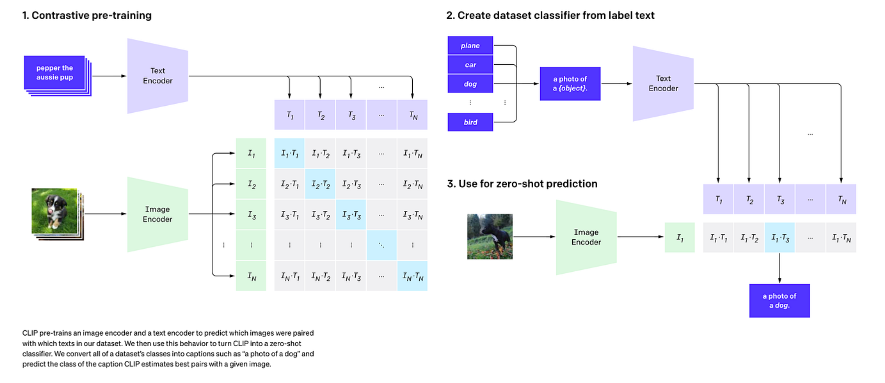
The basic logic of CLIP is illustrated in the figure above:
- Contrastive Pre-training: A batch contains N images and N text descriptions (paired). The Image Encoder produces \(I_1...I_N\), the Text Encoder produces \(T_1...T_N\), and an \(N \times N\) similarity matrix \(S_{ij} = I_i \cdot T_j\) is computed. The training objective is to maximize the similarity along the diagonal (correct pairs) and minimize it off-diagonal (incorrect pairs).
- Create classifier from label text: In traditional classifiers, the final layer's weight matrix = class parameters. In CLIP, the class text embeddings = class prototypes. For example, given three classes: "a photo of a dog," "a photo of a car," "a photo of a plane" — these sentences are passed through the text encoder to obtain 3 vectors, which become the classifier's weights.
- Zero-shot inference: Given a new image, the image encoder produces vector \(I\), its similarity to each class text vector is computed, and the class with the highest similarity is the predicted result.
The key to CLIP is not "a stronger visual backbone" but rather changing the task from "classification" to "alignment." It transforms "learning a classifier" into "learning a shared semantic space":
- The image encoder maps images to vectors \(v\)
- The text encoder maps text to vectors \(t\)
- Training objective: matching (image, text) pairs should have high vector similarity; non-matching pairs should have low similarity
Through this approach, a space that accommodates both visual semantics and linguistic semantics can be learned. Once this space exists, classification becomes a retrieval problem:
- Write all categories as sentences (prompts)
- Encode them into text vectors
- Let the image vector "find the most similar text"
In this way, classification becomes image-text similarity retrieval.
In summary, CLIP addresses the following problems:
- Open-vocabulary classification: Any class that can be described in text can be attempted (capability depends on training data coverage)
- Reduced transfer cost: No need to train a new classification head for each task
- Richer semantics: Since supervision comes from natural language, the granularity is finer — for example, the model learns the concept "red car" rather than just "car"
- Scalable supervision: Image-text pairs are far cheaper to obtain than fine-grained class labels
However, problems that CLIP does not solve include:
- CLIP performs alignment, not "locating where" — native CLIP has no localization or detection capability
- Limited compositional generalization — strong compositional reasoning like "a red cube to the left of a blue sphere" may not be robust
- Serious data noise and bias issues — internet image-text pairs are inherently noisy, with biases and shortcut learning
- Sensitivity to prompts — "a photo of a dog" vs "a dog" can produce very different results, which led to techniques like prompt engineering and prompt ensembling
ViT Architecture Case Study
Qwen2.5-VL-3B-Instruct
A simplified understanding of the architecture:
Input Image (H x W x C)
  |
Split into patches (P x P) --> N patches
  |
Linear projection to D-dim tokens  (N x D)
  |
Add positional embedding (+ optional [CLS])
  |
Transformer Encoder x L
  - (Window) Multi-head self-attention
  - MLP (SwiGLU/GELU)
  - Norm + residual
  |
Output visual token sequence (N x D) / or CLS for classification
After the input image is divided into patches of size P, each patch is encoded as an embedding of length D, and then fed as a sequence into the Transformer.
Reflections and Discussion
Why Does ViT Need Large Data?
ViT underperforms CNNs on small datasets — a phenomenon whose underlying cause is worth careful consideration.
The convolutional operation in CNNs is essentially a form of hard-coded prior knowledge:
- Local connectivity tells the model: "adjacent pixels are more correlated" — the model does not need to learn this from data
- Weight sharing tells the model: "the same pattern can appear anywhere in the image" — the model does not need to learn a separate detector for each position
In contrast, ViT's Self-Attention is global and unconstrained:
- Every patch can attend to any other patch; the model must learn on its own that "nearby patches are more correlated"
- Without the weight-sharing assumption, the model must discover translation equivariance by itself
- Knowledge that CNNs obtain "for free" must be learned by ViT from data
Therefore, when data is insufficient, ViT cannot learn good spatial priors and naturally underperforms CNNs. But when data is abundant, ViT is not constrained by CNN's inductive biases and can learn more flexible and powerful representations.
Is Inductive Bias a Blessing or a Curse?
There is no absolute answer to this question — it depends on data scale and task requirements:
| Scenario | Strong Inductive Bias (CNN) | Weak Inductive Bias (ViT) |
|---|---|---|
| Small data (< 10K) | Clear advantage | Severe overfitting |
| Medium data (ImageNet-scale) | Stable performance | Requires careful training (DeiT) |
| Large data (JFT/LAION-scale) | Tends to saturate | Continues to improve |
| Domain-specific tasks | High efficiency | May be overkill |
| General foundation models | Insufficient flexibility | Higher expressive capacity |
Looking at the trend, as data and compute continue to grow, models with weak inductive bias (such as ViT) have the advantage in terms of performance ceiling. However, in resource-constrained scenarios, CNNs' efficiency advantage remains significant.
Will ViT Completely Replace CNNs?
In the short term, no. Here is why:
- Resource efficiency: CNNs still have an unmatched efficiency advantage on edge devices and mobile platforms. MobileNet-series CNNs can run in real-time on phones, while ViT models of comparable accuracy require significantly more computation.
- Small data scenarios: In fields such as medical imaging and industrial inspection where data is scarce, CNN's inductive biases remain valuable.
- Hybrid architectures: In practice, an increasing number of models adopt hybrid CNN + Transformer architectures (e.g., CoAtNet, EfficientFormer), combining the strengths of both.
In the long term, the trend is indeed shifting toward Transformers:
- The paradigm of large-scale pre-training + fine-tuning naturally suits ViT
- ViT shares the same architecture as language models, facilitating multimodal unification (e.g., CLIP, GPT-4V)
- Variants such as Swin Transformer have already surpassed CNNs in traditional CNN strongholds like detection and segmentation
A Deeper Perspective
From the perspective of the "No Free Lunch" theorem, no single architecture is optimal for all tasks. ViT's success is more attributable to our entering the era of "large data + large models" than to Transformers being mathematically superior to convolutions. If a more efficient global modeling mechanism than Self-Attention emerges in the future, ViT could similarly be superseded. Architectural evolution is always about finding the optimal balance among efficiency, expressiveness, and inductive bias.