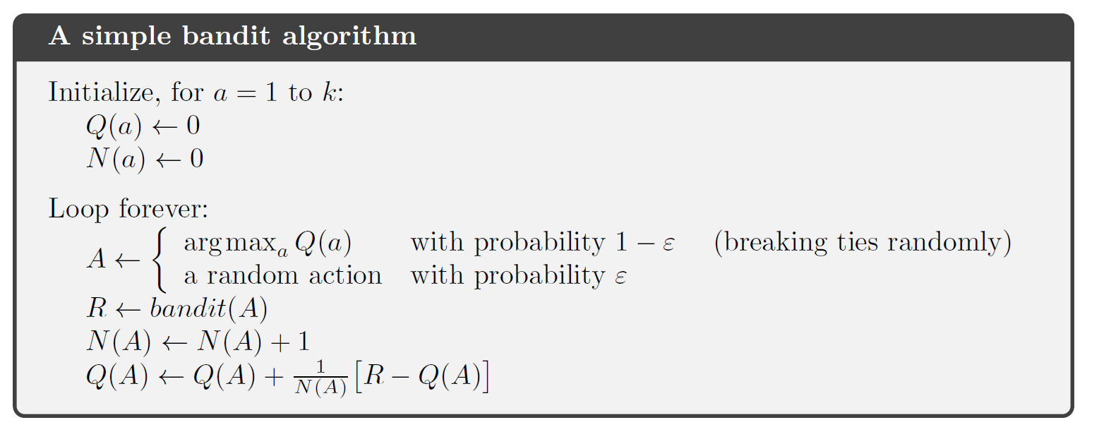
Multi-armed Bandits
2.0 Introduction
Starting from Chapter 2 on Multi-armed Bandits through Chapter 8 on Planning and Learning with Tabular Methods, the author collectively categorizes this portion as "Part I: Tabular Solution Methods" of the book.
In the previous chapter, we outlined the historical development of reinforcement learning and the importance of tabular solution methods to the rise of modern reinforcement learning. Tabular solution methods represent the simplest forms of nearly all core reinforcement learning ideas: when the state and action spaces are sufficiently small, approximate value functions can be represented as arrays, or tables. In such cases, these methods can often find exact solutions — namely the optimal value function and optimal policy.
Beginning in Chapter 9, the book introduces scenarios where only approximate solutions can be found. As mentioned in the historical overview of the previous chapter, modern reinforcement learning originated from tabular methods, but large-scale real-world applications only became feasible when combined with artificial neural networks, at which point reinforcement learning demonstrated astonishing results.
In Part I, we will study the following topics:
| Chapter | Content | Key Concepts |
|---|---|---|
| 2 | Bandit Problems | ε-greedy |
| 3 | Markov Decision Processes | Bellman Equation, Value Functions |
| 4 | Dynamic Programming | Environment Model |
| 5 | Monte Carlo Methods | Experience-based Estimation |
| 6 | Temporal-Difference Learning | Bootstrapping |
| 7 | Combining Monte Carlo and TD | TD(λ), Multi-step Updates |
| 8 | Combining TD and Model-based Methods | Dyna Architecture |
In this chapter, we primarily study a relatively simple yet highly important concept in reinforcement learning: the trade-off between exploitation and exploration. One of the most important distinctions between reinforcement learning and other types of learning is that RL uses training information that evaluates the actions taken, rather than instructs by providing the correct action. Clearly, if the environment can only evaluate how good an agent's actions are without telling the agent which action is correct, then the agent must actively explore — otherwise it might never discover whether better actions exist. The fundamental reason is that the information available to the agent is always in a state of partial observability; it is incomplete. Therefore, the agent must continuously learn through trial and error to discover which actions yield high rewards, and gradually find the optimal policy. Since the environment cannot provide instructions, active exploration is the only path to finding the optimal policy.
For example, imagine you are playing Super Mario. Instructive feedback would directly tell you based on training data: on this screen, you should jump to the right. You just follow the instruction because there is a clear directive. This is an important characteristic of supervised learning. In this case, regardless of what you do, the system does not evaluate your action — it simply tells you: in this state, the correct action is to move right.
In reinforcement learning, however, you control Mario, press an action button, and the system tells you: you just scored 200 points. The system does not tell you what the maximum possible score is. Therefore, you can only keep playing, over and over, to see whether your score can keep improving. In this case, your action is what the system focuses on — the system knows how to evaluate it, but cannot tell you the correct answer.
2.1 The K-armed Bandit Problem
In this chapter, we will use a concrete example to illustrate how an evaluative system operates. This example is a simplified version of a reinforcement learning problem that lacks associativity. Associativity means that action selection must be linked to the current situation or state. For instance, when an agent explores a maze, it obviously takes different actions at different positions. When there is a wall to the left, the agent clearly cannot continue moving left; when there is a wall to the right, it clearly cannot move right. In this case, which direction to move (action) is influenced by the current position (state) — they cannot be considered independently. This is the associative case, and it is a characteristic that all real-world problems naturally possess.
To simplify the problem, let us first discuss a nonassociative example. Imagine the following scenario: you have a slot machine in front of you:

This slot machine has a lever that you can pull, and the screen will spin:

If the symbols in the center of the screen are all the same when it stops, you win!
The author once played this machine in Las Vegas, spent ten dollars, won twenty, and then bought Starbucks with a friend. The author personally does not enjoy gambling — the most gambling they had ever done before was buying ten-dollar scratch cards, and they often won twenty dollars.
Back to the topic. Now suppose you are an avid gambler wanting to apply your knowledge to this problem. What would you think about first? Indeed, most people would first look around at the different machines and decide which one to use, since that is probably the only decision you can make in a slot machine game. Suppose there are now k machines in front of you, and you can choose any one to pull. Your goal is to find the machine with the highest payoff. This is the k-armed bandit problem:

Let us examine this problem systematically: your goal is essentially to maximize the expected cumulative reward over a certain period — for example, maximizing the total reward obtained over 1000 actions (in reinforcement learning, we call 1000 actions 1000 time steps).
Now, suppose each action a has an expected reward (or mean reward), which we call the value of that action.
Let At denote the action selected at time step t, and Rt denote the reward received. Then the "true" value of an action a can be written as:
This formula means: the expected reward when action a is selected. For those who may not have much mathematical background, here is what each element means:
- a — the action, i.e., the action actually selected
- At — the action taken at time step t; At = a means the action taken is a
- Rt — the reward received at time step t
- | — conditional symbol; Rt | At = a means the reward obtained given that action a is selected
- \(\mathbb{E}[ X | Y]\) — conditional expectation; the expected value of X given condition Y
- \(\doteq\) — definitional symbol, indicating this is a definition rather than an equation
- \(q_*\) — the asterisk * denotes optimal; q represents the expected reward; \(q_*(a)\) is the expected reward when action a is selected
A quick review of expected value: the expectation refers to the sum of each possible outcome of an experiment multiplied by its probability. Note that \(q_*(a)\) here refers to the true value; the next section will explain how to estimate it.
2.2 Action-Value Methods
We cannot obtain the true value right away; we can only estimate it through repeated trials. A very intuitive estimation method is to simply take the average of past rewards received when that action was taken — the sample-average method:
where:
- \(\mathbb{1}_{\text{predicate}}\) is an indicator function that takes the value 1 when the condition is true and 0 otherwise.
- Qt(a) is the action-value function.
If the action has never been selected, the denominator is 0, so in this case we need to define Qt(a) for this special case — typically set to 0. By the law of large numbers, as the denominator approaches infinity, \(Q_t(a)\) converges to the true value \(q_*(a)\).
Now, at any given moment when facing k slot machines, you can use the sample-average method described above to compute the estimated value for each action. Among these values, you can take two kinds of actions:
- Greedy action: select the action with the highest value. Because it exploits the value information, we call greedy action exploiting.
- Non-greedy action: select an action that does not have the highest value, typically by choosing randomly. Because it does not exploit the value, we call this exploring.
In this task, because the estimated values are computed from samples, they only reflect outcomes that have already occurred and are therefore partial. If we do not want to miss potentially better options, exploration is essential. Initially, exploration may yield lower rewards, but once a better action is found, it can be exploited repeatedly, thereby increasing long-term returns. Since we cannot simultaneously explore and exploit, there exists a complex trade-off between the two, which is a core aspect of reinforcement learning.
When considering this trade-off, we generally account for:
- The precision of current value estimates
- The uncertainty of each action
- The number of remaining time steps
In this book, our focus is not on the exploration-versus-exploitation trade-off itself, so we consider only simple balancing strategies. When we base action selection on these values, we call such methods action-value methods. In general, a complete action-value function also includes the state, i.e., \(Q_t(s,a)\), but since there is no state in the bandit problem, we discuss only the simplified action-value function here.
Now we can define the action selection rule. If we always select only the action with the highest estimated value — the greedy action — we can write:
where \(\arg\max_a\) denotes the action a that maximizes Q_t(a).
But this clearly will not work. We obviously need to incorporate exploration. A common approach is to make greedy selections most of the time, but occasionally select a random action with a small probability ε (epsilon). We call this the ε-greedy method.
As the number of steps approaches infinity, every action will eventually be tried infinitely many times, so each estimated value converges to the true value, and the probability of selecting the optimal action converges to 1-ε — meaning the optimal action is almost always selected. However, such asymptotic guarantees do not fully reflect the method's practical effectiveness under a finite number of steps.
2.3 Multi-armed Bandit Simulation
Let us now design a simulation experiment. The textbook provides a 10-armed testbed to evaluate and compare greedy and ε-greedy strategies.
Below, we replicate the experiment from the book. The key experimental setup is as follows:
- k=10, simulating 10 slot machines (or equivalently, a 10-armed bandit)
- The true rewards \(q_*(a)\) for all 10 machines are predetermined (details below); these rewards are hidden and invisible to the agent
- At each action selection, random noise is added to the true reward
Once the testbed is set up, it effectively simulates a reinforcement learning environment. We can then apply reinforcement learning algorithms to let the agent learn in this environment and finally evaluate the results. In this example, we will gain an initial understanding of how to set up a simple simulated environment, run tests, and perform evaluation.
First, before starting the experiment, let us describe the testbed setup. k=10 is straightforward — 10 machines or equivalently a 10-armed bandit.
The true rewards are generated from a standard normal distribution:
This means that the "quality" (mean reward) of each action is randomly drawn from a distribution with mean 0 and variance 1.
For each action, the actual reward received upon execution is subject to noise. We set the actual reward Rt as:
In simple terms, we first generate 10 true reward values from the standard normal distribution (mean 0, variance 1); then for each action, the actual reward is sampled using the action's true reward as the mean, with variance 1.
We can set up this distribution in Python:
import numpy as np
import matplotlib.pyplot as plt

# 设置随机种子
np.random.seed(42)

# 模拟一个 10 臂赌博机
k = 10

# 为每个动作生成真实平均奖励 q_*(a)
q_star = np.random.normal(loc=0.0, scale=1.0, size=k)

# 生成每个动作的实际获得的奖励样本
rewards = []  # 最终是一个长度为10的列表,每个元素是该动作的1000次奖励
for i in range(k):
    q = q_star[i]  # 第i个动作的真实平均值
    reward_samples = np.random.normal(loc=q, scale=1.0, size=1000)  # 模拟拉1000次
    rewards.append(reward_samples)

# 创建小提琴图来展示奖励分布
plt.figure(figsize=(12, 6))
plt.violinplot(rewards, showmeans=True, showextrema=False)
plt.axhline(0, color='gray', linestyle='--')
plt.xticks(np.arange(1, k + 1))  # 标出动作编号
plt.xlabel("Action")
plt.ylabel("Reward Distribution")
plt.title("Reward Distributions for 10-Armed Bandit Actions (Using For Loop)")
plt.grid(True)
plt.tight_layout()
plt.show()
Because a random seed is set, we are effectively using a fixed set of pseudorandom numbers. The reason for using the normal distribution is that rewards are concentrated around a certain value (e.g., the mean), with occasional fluctuations (good luck / bad luck), and the normal distribution is mathematically convenient. Sampling 1000 actual rewards for each action produces the following result:
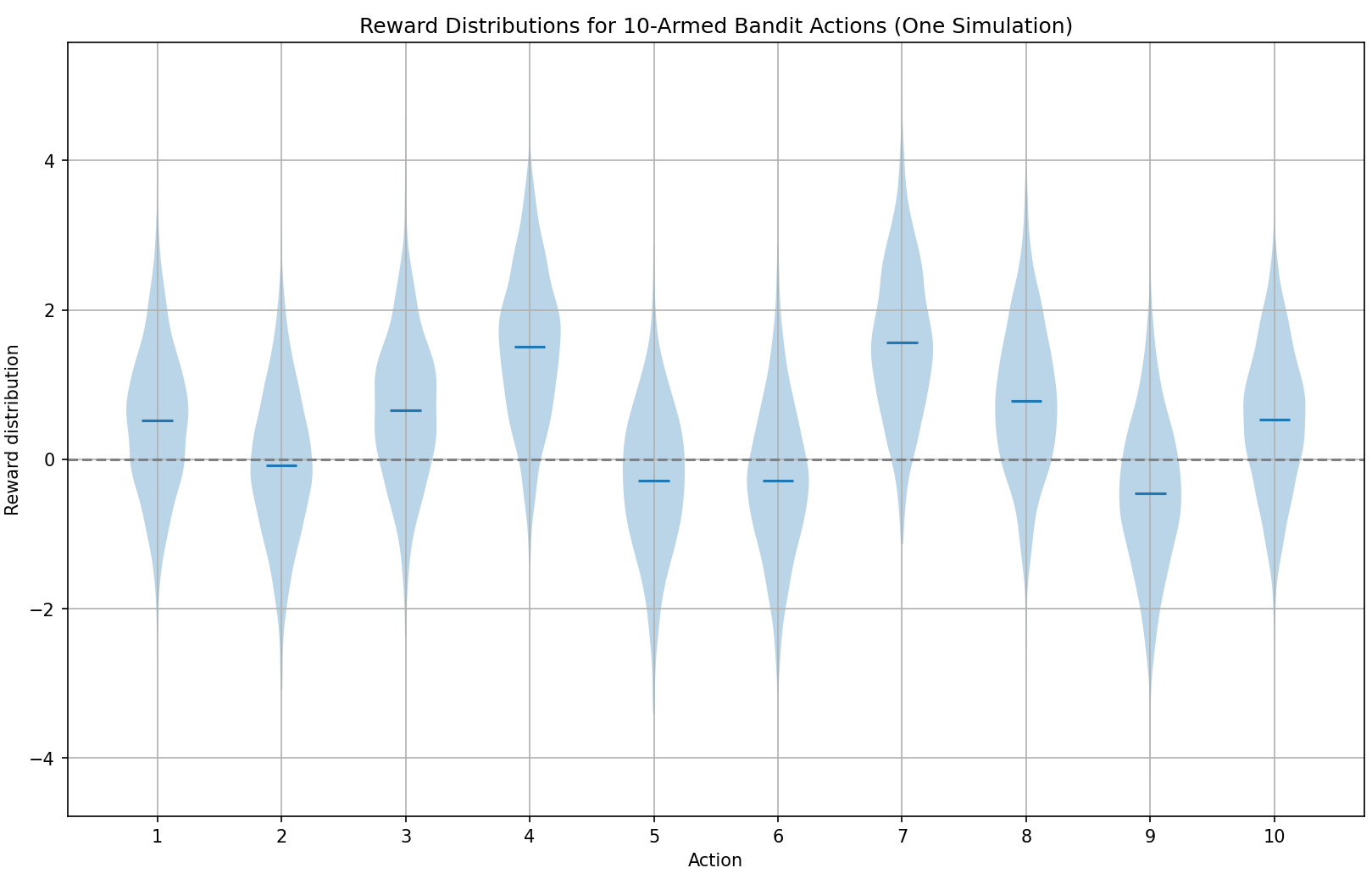
This is called a "violin plot," which intuitively shows the distribution of the true q-values under this testbed configuration. In the actual tests that follow, the agent cannot observe any of this — it can only adjust its Q-value estimates based on the actual rewards received. When the Q-values converge, we can see whether the agent has found the correct answer.
Now that we know how the environment distributes rewards, we can begin the experiment. Suppose the agent initially estimates all 10 action Q-values as 0. In the first round, regardless of the agent's chosen ε (in our discussion here, we treat pure greedy as the case where ε = 0), the agent obviously must randomly select one action when facing 10 equal Q-values. Randomly selecting one when Q-values are tied is the standard approach.
Regardless of which action the agent randomly selects, the environment returns a reward (the noisy reward described above). Here we can simply update the Q-value for action a using the sample-average update method, where Q(n+1) is the action value estimated after observing the first n rewards:
This method is impractical for actual experiments and programming because it consumes too much memory. Obviously, from a programming perspective, we always set up a loop and update a variable incrementally within the loop (e.g., the very common for i in... i+=1). Similarly, the Q-table update can be done the same way:
This formula holds even when n=1, in which case Q2 = R1 for any Q1.
We can now set up a test environment to compare how the agent performs under different ε values in finding the highest-reward bandit.
Based on the above formula and our reward setup, writing as we read, we can draft the overall program framework as follows:
伪代码:多臂老虎机测试

def reward(agent选择了老虎机a):
  设置该函数来按照上面我们已经讨论过的规则,将对应老虎机的奖励返还给agent
  k = 10,代表10个老虎机
  按照标准正态分布设置十个老虎机的真实奖励q*
  然后根据导入的参数老虎机k(代表agent选择的对应的老虎机)返回一个带噪音的Rt
  Rt(a) = 正态分布(以q*为中心,方差为1)
  return Rt(a)

def agent:
  agent就是强化学习智能体,该智能体将和环境交互
  agent初始维护一个值全为0,长度为k=10的Q表
  Q = [0] * 10
  然后agent在每次的选择中,将根据Q表中的最大值来决定选择哪个动作at:
  (1)在Q表中找到最大的值,返回其对应的index,即选择动作;如果有多个最大值,则随机选择一个
  (2)调用reward(a),获得对应的奖励
  (3)根据实际的反馈,更新Q值,这里按照样本平均更新法来更新

def main:
  接着我们进行2000次试验,在每次试验中进行1000个时间步的运行:
    agent和环境交互,以ε的概率随机选择,以1-ε的概率按照agent中定义的方式选择
    选择后更新Q值
  试验结束后绘制图表,展现1000个时间步在2000次试验中的平均奖励,以及选择最优动作的百分比(理想状况下ε策略将按照1-ε的概率选择最优动作)
This approach is clearly not elegant — it merely restates the reward and agent concepts we just learned. We can refine the key points using an object-oriented design. The entire process involves only two objects: the slot machine itself (environment) and the agent. So the pseudocode can be refined to:
class 老虎机:
    def init():
        初始化k=10
    按照标准正态分布生成上述k个动作的真实平均奖励q*

    def 实际奖励(选择的动作a):
    reward = 以动作a的真实平均奖励q*为中心,方差为1的正态分布中的值
    return reward

class Agent:
    def init(epsilon):
    初始化epsilon
    初始化Q表(按照k的值设置对应数量的初始值,这里设置为0)

    def 动作选择():
    生成一个随机数
    if 该随机数小于epsilon:
        进行ε-greedy选择一个随机动作
        return 动作a
    else:
        进行greedy,选择一个值最大的动作,如果都一样则从中随机选择一个
        return 动作a

    def 更新Q表(动作a,实际奖励q):
    根据动作a和实际奖励q,更新Q(a)

def main():
    agent = Agent(epsilon=0/0.01/0.1)
    老虎机 = 老虎机()
    进行1000次循环:
    动作a = agent.动作选择()
    奖励q = 老虎机.实际奖励()
    agent.更新Q表(动作a, 奖励q)

if self = _init_:
    新建三个Q表,用来存放2000次试验下不同epsilon值的平均值
    遍历三种epsilon值:
        进行2000次试验:
        main()
Now it looks more like something. Let us fill in the details. In subsequent notes, I will skip the above process and directly present the final detailed pseudocode. The verbose treatment here is intended to help those who are not very experienced with programming (there are increasingly many people studying AI who are not skilled at coding — this is normal, since many focus primarily on mathematics! But reinforcement learning is very well-suited for practical applications, especially when combined with robotics, so there will be quite a bit of programming! That said, the author believes that for studying reinforcement learning, being able to write pseudocode is sufficient, since RL code is generally not very long. The most important things are the policy and environment design — the actual code implementation can be delegated to ChatGPT!)
When writing the pseudocode for the entire program, the most critical aspect is object-oriented design. If you have not yet learned about object-oriented concepts, you can quickly go through a Python/Java online tutorial — in about an afternoon you can understand the main features such as objects, inheritance, overriding, etc. Generally speaking, the author believes that being able to write pseudocode at the level shown below is sufficient for reinforcement learning programming:
# 多臂老虎机测试伪代码
class 老虎机:
    def __init__():
        k = 10  # 动作数
        # 按照标准正态分布生成 k 个动作的真实平均奖励 q*
        q_star = [从 N(0, 1) 中采样得到的长度为 k 的列表]
        # 记录当前环境下的最优动作索引
        best_action = argmax(q_star)

    def 实际奖励(选择的动作 a):
        # 根据动作 a 的真实平均值 q_star[a],从 N(q_star[a], 1) 中采样
        reward = 从 N(q_star[a], 1) 中采样得到的标量
        return reward


class Agent:
    def __init__(epsilon):
        # 探索概率 ε
        self.epsilon = epsilon
        # 初始化 k 个动作的估计值 Q[a] = 0
        self.Q = 长度为 k、全零的列表
        # 初始化每个动作被选择的计数 N[a] = 0
        self.N = 长度为 k、全零的列表

    def 动作选择():
        随机数 = 从 [0, 1) 均匀采样
        if 随机数 < epsilon:
            # 以 ε 的概率随机探索
            a = 在 0 到 k-1 之间随机选一个动作索引
            return a
        else:
            # 以 1 - ε 的概率进行贪心选择
            max_Q = max(self.Q)
            # 找出所有 Q[a] == max_Q 的索引列表
            candidates = [所有满足 Q[a] == max_Q 的索引]
            # 如果有多个相同的最大值,从中随机选择一个
            a = 在 candidates 列表中随机选一个索引
            return a

    def 更新Q表(动作 a, 实际奖励 r):
        # 计数加一
        N[a] += 1
        # 样本平均法更新:Q[a] ← Q[a] + (1 / N[a]) * (r - Q[a])
        Q[a] = Q[a] + (r - Q[a]) / N[a]


def main():
    # k = 10,steps = 1000
    # 在 main 中只跑一次环境交互(一个试验/一次序列)
    agent = Agent(epsilon=0 或 0.01 或 0.1)
    env = 老虎机()
    # 用于记录单次试验中每个时间步 t 的奖励和最优动作命中情况
    rewards_list = 长度为 1000、初始值全零的列表
    optimal_action_flags = 长度为 1000、初始值全零的列表

    for t in range(1000):  # 进行 1000 个时间步
        a = agent.动作选择()
        r = env.实际奖励(a)
        agent.更新Q表(a, r)

        rewards_list[t] = r
        if a == env.best_action:
            optimal_action_flags[t] = 1

    return rewards_list, optimal_action_flags


if self = _init_:
    k = 10
    steps = 1000
    runs = 2000
    epsilons = [0, 0.01, 0.1]

    # 用于累计所有 runs 次试验中,每个 ε 对应的 1000 个时间步的总奖励
    总奖励 = 一个字典,键为 ε,值为长度为 1000 的全零列表
    # 用于累计最优动作命中次数
    总最优命中 = 一个字典,键为 ε,值为长度为 1000 的全零列表

    # 遍历三种 ε
    for ε in epsilons:
        for run in range(runs):
            # 每个 run 都重新执行一次 main,得到该次序列的 rewards 和 optimal flags
            rewards_list, optimal_flags = main()
            # 累加到对应 ε 的"总奖励"和"总最优命中"中
            for t in range(steps):
                总奖励[ε][t] += rewards_list[t]
                总最优命中[ε][t] += optimal_flags[t]

    # 计算平均值:每个ε下,每个时间步的平均奖励 和 最优动作命中率(%)
    平均奖励 = 一个字典,键为 ε,值为长度为 1000 的列表
    最优命中率 = 一个字典,键为 ε,值为长度为 1000 的列表

    for ε in epsilons:
        for t in range(steps):
            平均奖励[ε][t] = 总奖励[ε][t] / runs
            # 将命中次数转换为百分比
            最优命中率[ε][t] = (总最优命中[ε][t] / runs) * 100

    # 最后可以将 平均奖励 和 最优命中率 用于绘图或表格展示
    # 此处省略具体绘图代码,可以直接告诉ChatGPT用 matplotlib 画就行了
Following the pseudocode above, you can send it directly to ChatGPT, have it write the actual code, and then run it in a Python environment. The specific code can be found in the Code Appendix at the end of this section or in my GitHub repository. Unless there is a special reason, just look in the appendix, since the GitHub repo contains not only notes and code files but also some other files (such as those needed to render this notebook wiki), which can be a bit cluttered.
See Appendix Code 2.1 for the specific code.
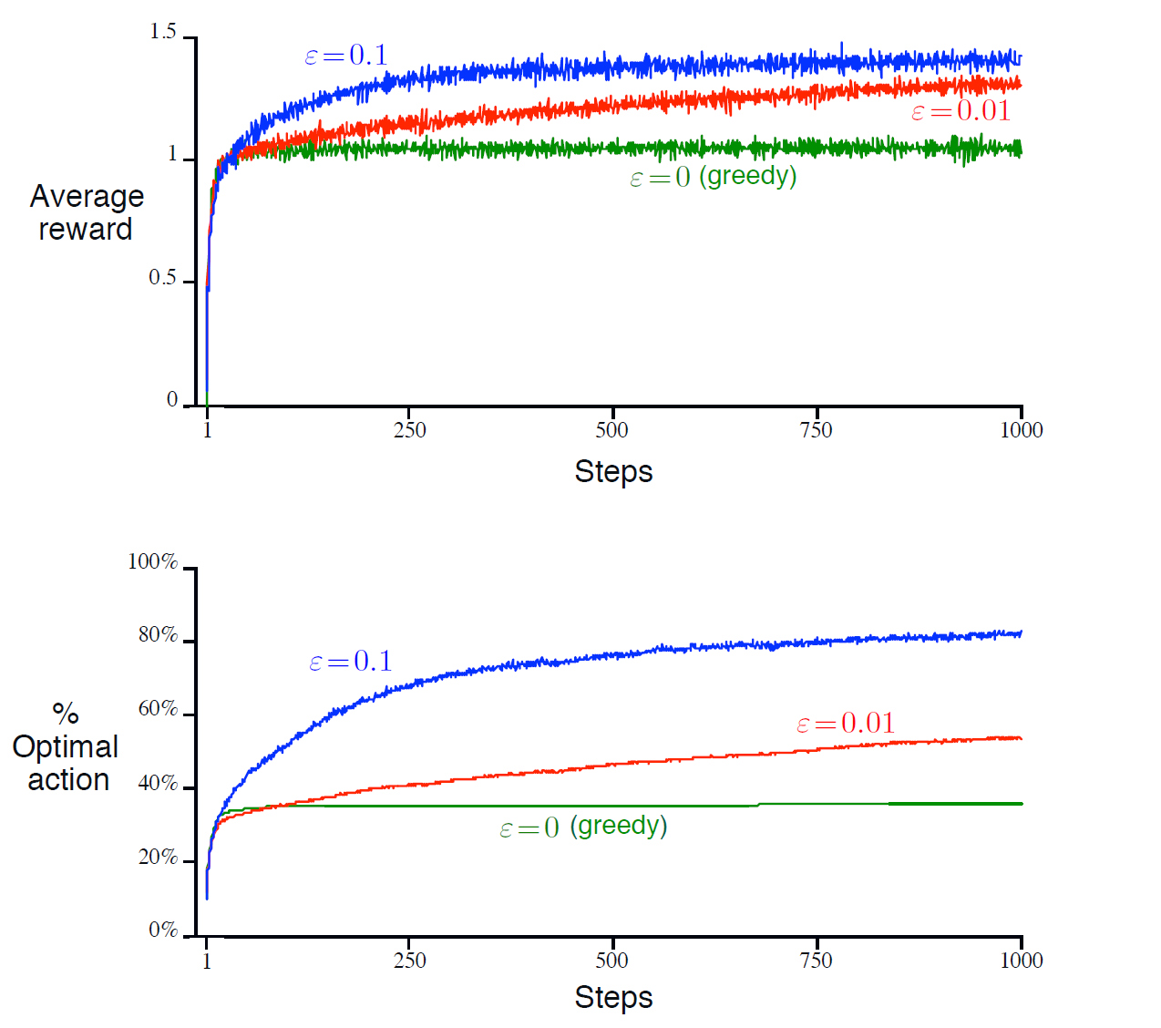
Running the code produces the following result:
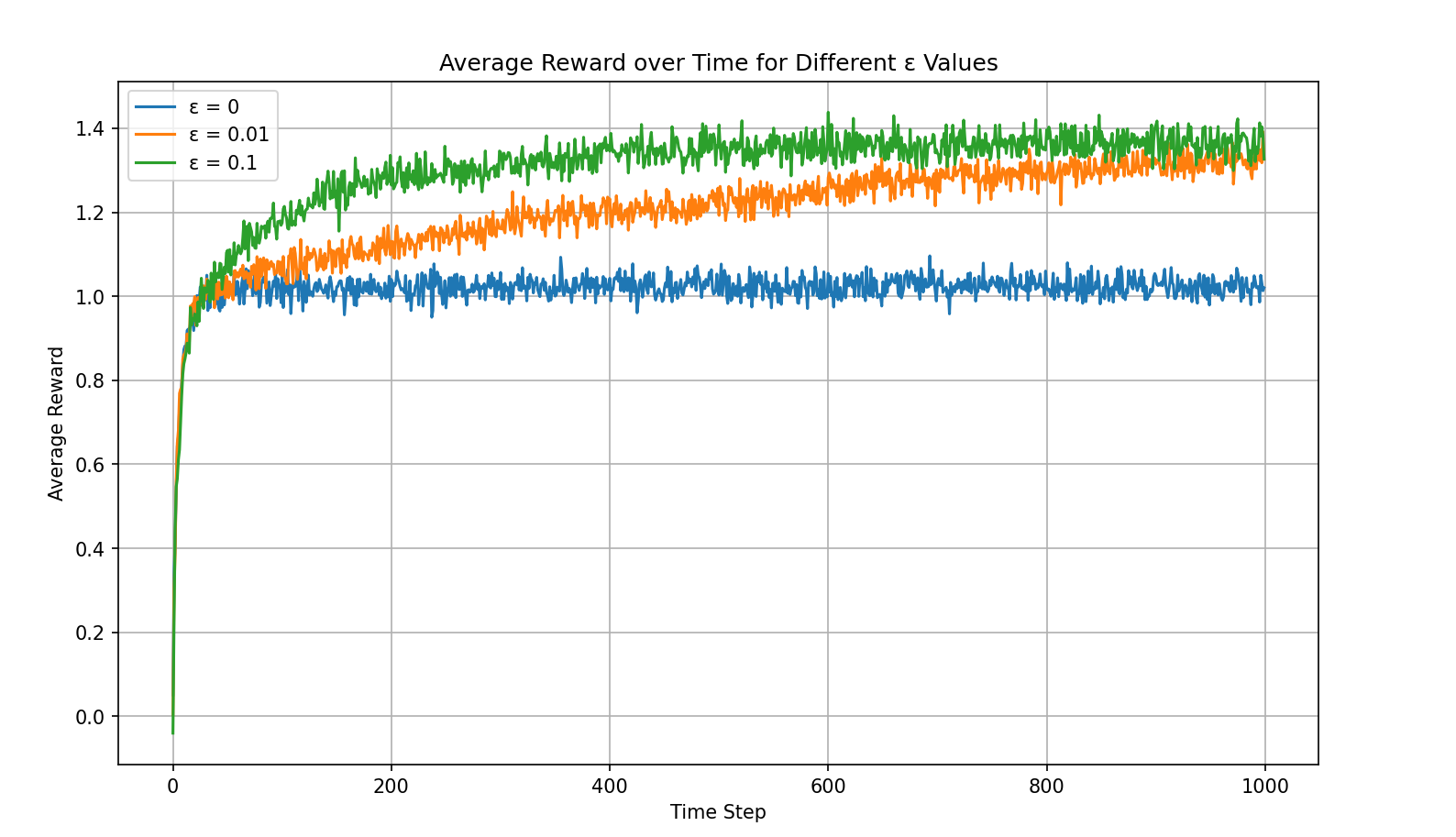
This figure shows the average reward across 2000 trials over 1000 time steps for three ε strategies. This average reward over time plot is one that nearly every RL task must produce — it most intuitively shows the agent's learning trend.
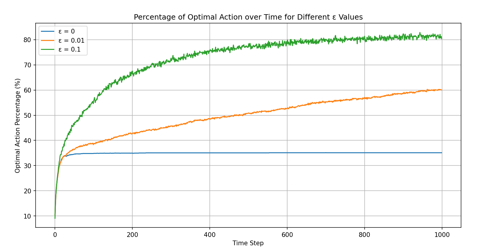
This figure is the optimal action selection rate plot, used for analyzing exploration versus exploitation.
From the two figures above, it is clear that among the three strategies, ε=0.1 performs the best. Let us analyze these two figures in more depth:
- The pure greedy strategy converges very quickly and gets stuck in a local optimum.
- ε=0.1 converges to approximately 1.5, which is close to the theoretical optimal value of 1.54. This can be proved mathematically — see Math 2.1 in the appendix.
- The optimal action selection rate for ε=0.1 does not converge to the theoretical optimum of 91% (during random exploration there is a 10% chance of selecting the optimal action, so the theoretical value is 90% + 10%*10%). This is a very interesting point. The reasons are multifaceted, since the figure shows the average across 2000 trials, so it is possible that in some trials the agent never found the best machine. The author did not investigate the specific cause further. If any interested reader discovers a precise reason, or finds an ε value that converges to the theoretical optimum, please let the author know — it would be greatly appreciated!
Exercises for this section: see Exercise 2.2 and Exercise 2.3 in the appendix.
2.4 Incremental Implementation
In the previous section, we already introduced a rather clever update formula for Q-values:
This formula is formally introduced in this section of the book, but we already used it in the previous chapter to complete the code and exercises. This type of formula is called an incremental formula. Incremental Implementation appears multiple times in this book, and its general form is:
where:
- \(\text{Target} - \text{OldEstimate}\) represents the "error" in the current estimate
- \(\text{StepSize}\) represents the step size (in this example, \(\frac{1}{n}\))
The core idea is to take one step at a time rather than jumping directly to the endpoint (the target value). Why do we do this? Because we do not know the true target value — we can only observe a target value that most likely contains noise. For instance, the reward may be random, state transitions uncertain, data imperfect, and so on. Therefore, we cannot directly set the estimate to the target value; instead, we must gradually approach it. This incremental learning approach adapts flexibly to environmental changes and is not severely affected by any single outlier.
Here, the book summarizes the bandit algorithm we wrote ourselves in the previous section. Q(a) is the Q-value, and N(a) is the number of times action a has been selected. If you carefully wrote the code in the previous section, this should look very intuitive and clear, so we will not elaborate further:
2.5 Tracking a Nonstationary Problem
Now consider the following situation: if the environment is slowly changing, we must consider how to adapt to such changes. Using the formula from Section 2.4 is clearly inappropriate, because rewards from both early and recent time steps are weighted equally in the formula.
In RL, most problems are actually nonstationary. In such cases, we should find a way to assign greater weight to more recent rewards. Here we introduce a very common method: using a constant step-size parameter. That is, we change the formula from Section 2.4:
to:
Here α is the constant step-size parameter, a constant between 0 and 1. It is easy to see that Q(n+1) becomes a weighted average of past rewards and the initial estimate Q1. Through mathematical derivation:
As can be seen, the weight of the earliest reward (at t=1) decreases exponentially over time (with exponent 1-α). For this reason, this method is also called exponential recency-weighted average.
According to stochastic approximation theory, for convergence to be guaranteed, the following two conditions must be satisfied:
We can see that the sample-average method (\(\alpha_n(a) = \frac{1}{n}\)) satisfies both conditions; however, the constant step-size method does not satisfy the second condition, meaning the Q-value will keep fluctuating with the latest reward indefinitely. Although it cannot converge, because nonstationary problems dominate in reinforcement learning, this method is generally adopted in practice.
An important point to note here (which is asked about in Exercise 2.7): the sample-average method is unbiased, while the constant step-size method is biased. In statistics, if the expected value of an estimator equals the true value being estimated, we say the estimator is unbiased. That is, if \(X\) is the true value we want to estimate (e.g., the expected reward of some action) and \(\hat{X}\) is our estimate (e.g., Qn), then if \(\mathbb{E}[\hat{X}] = X\), we say the estimate is unbiased. The reason we discuss this here is that if a method is unbiased, then after sufficient learning, the estimate will on average equal the true value. Unbiased methods are suitable for stationary environments, such as the bandit problem; biased methods are suitable for nonstationary environments, as they can quickly adapt to new changes (because recent rewards receive higher weight).
Summary: Through this section, we have now mastered the following two Q-value update formulas:
Exercises for this section: see Exercise 2.4 and Exercise 2.5.
2.6 Optimistic Initial Values
This section discusses the concept of Optimistic Initial Values.
In the previous section, we mentioned that the constant step-size method is biased. In reinforcement learning, this bias is not a problem and can sometimes even be very helpful. The only drawback is that the user needs to think about how to set the initial values, because the initial value Q1 term in the constant step-size method can never be fully eliminated. In Code 2.1 and Code 2.2, we set all initial values to 0. What would happen if we set the initial values to 5 in both experiments?
Clearly, no reward will ever reach 5. Therefore, after the agent selects an action and updates the Q-value, those actions that were not selected will naturally appear to have higher values. Consequently, this design ensures that all actions are visited. This method is called the optimistic initial values method.
We only need to slightly modify the Code 2.1 code to obtain the following comparison results (see Code 2.3 Optimistic Initial Values for the running code):
As can be seen, the optimistic initial values method, even using a greedy strategy with epsilon=0 and performing poorly at the beginning, surpasses the ε-greedy strategy with initial values of 0 at around step 200 and converges to a better level.
However, if the task changes (e.g., in a nonstationary environment), we may need to explore again. The starting point occurs only once, and we should not focus on it too much. Nevertheless, this clever initialization technique is highly effective in many practical applications. The purpose of this section is simply to remember that such a special technique exists.
See the Exercise appendix section for Exercise 2.6 and Exercise 2.7.
2.7 Upper-Confidence-Bound Action Selection
In ε-greedy, we cannot treat all non-greedy options equally and explore thoroughly. If non-greedy actions have the potential to be optimal, and we prioritize exploring those with higher potential, we can improve the efficiency of the exploration-exploitation trade-off — that is, we conduct more strategic exploration (rather than blind exploration).
This section introduces a method called Upper-Confidence-Bound (UCB) action selection, which can explore more strategically and adaptively reduce exploration frequency. Consider the following formula:
where t is the time step, Nt(a) is the number of times action a has been selected up to time t, and c > 0 is a parameter controlling the degree of exploration. Q(a) represents the current estimated value of action a, i.e., exploitation; the right half represents the exploration bonus term, used to estimate the degree to which the current action "might be underestimated" — that is, the upper bound of uncertainty. This is the origin of the name "upper confidence bound."
Note that if Nt(a) = 0, meaning an action has never been selected, then having it in the denominator makes the term infinitely large. In this case, the action is considered maximizing. This ensures that all unexplored actions are forced to be explored. In practice, actions with Nt(a) = 0 can be executed first to avoid division-by-zero errors.
The idea behind UCB action selection is that if action a is selected more frequently, its uncertainty decreases; conversely, if action a has not been selected, then with the denominator not increasing while the numerator \(\ln t\) increases, the overall uncertainty grows. Meanwhile, the coefficient c represents the confidence level.
As time increases, actions with low estimated values that have been frequently selected will see their weights decrease over time. Intuitively, UCB's action selection logic works as follows:
| Action Situation | UCB Value | UCB Strategy |
|---|---|---|
| High estimate + low exploration term | Large | Frequently selected |
| Low estimate + frequently selected (confirmed bad) | Small | Gradually eliminated |
| Low estimate + rarely selected (uncertain) | May increase | Selected when possible |
We can run a simple experiment; see Code 2.4 UCB for the experimental code:
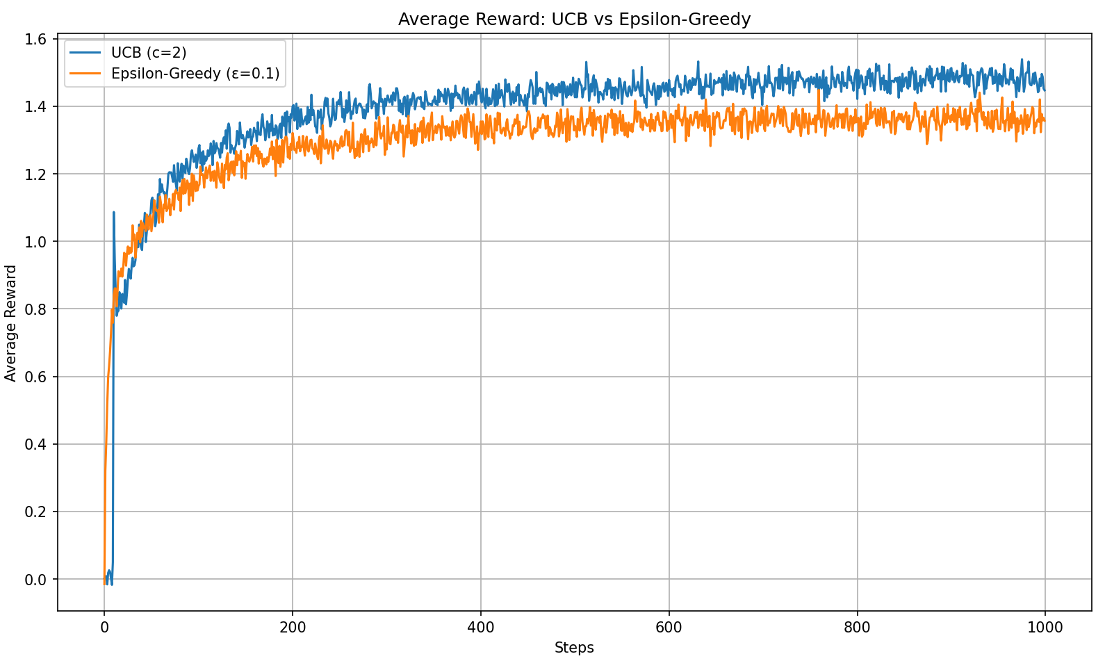
As can be seen, in the 10-armed bandit test, UCB performs better than ε-greedy. However, the book also points out that UCB is more difficult to generalize to general reinforcement learning problems beyond bandits. The main difficulties include:
- UCB has difficulty handling nonstationary problems
- UCB has difficulty handling large state spaces
Therefore, UCB has limited practical applicability and can be viewed as an optimization specific to the bandit problem.
See the Exercise appendix section for Exercise 2.8.
2.8 Gradient Bandit Algorithms
In the previous section, we introduced the UCB (Upper-Confidence-Bound) method, which selects actions by combining the current action-value estimate with uncertainty (typically measured by the log ratio of time steps to action selection counts). This method selects a deterministic action with the highest potential upper bound at each step, thereby achieving a trade-off between exploration and exploitation.
In this section, we introduce another method that also considers the potential of different actions but adopts a fundamentally different strategy: Gradient Bandit Algorithms. Unlike the UCB method, it does not compute action-value functions. Instead, it learns a preference value for each action and generates a probability distribution based on these preferences for sampling, thereby performing stochastic policy selection. This approach not only possesses greater generality (e.g., extensible to policy learning, continuous action spaces, etc.) but can also adapt to nonstationary environments through appropriate design (e.g., using a fixed step size and baseline).
This approach is called a policy-based method in reinforcement learning, while the methods studied in previous sections that estimate action values are called value-based methods. What this section introduces is one of the simplest policy-based methods, or equivalently, one of the simplest policy gradient methods.
Let us examine this method. First, we consider learning a numerical preference for each action \(a\), denoted \(H_t(a) \in \mathbb{R}\). The larger the preference value, the more frequently that action is selected. Note that these preferences themselves carry no meaning about rewards. What matters is the relative preference between actions.
In other words, this method does not need to directly estimate values; instead, it learns preferences for each action and then selects actions according to a probability policy. For example, if all actions have a preference of 1000, then there is no relative preference difference among them, and under this method, the action probabilities are unaffected. The action selection probability is determined by a soft-max distribution (e.g., Gibbs or Boltzmann distribution) as follows:
where \(\pi_t(a)\) denotes the probability of selecting action a at time t. Initially, all action preferences are equal, so each action is selected with equal probability.
Note: The book inserts a mathematical proof exercise (Exercise 2.9) here; see the Exercise appendix section for details.
For soft-max action preferences, there is a natural learning algorithm based on stochastic gradient ascent. At each step, after selecting action At and receiving reward Rt, the action preferences are updated as follows:
where:
- \(\alpha>0\) is the step-size parameter
- \(\bar{R}_t \in \mathbb{R}\) represents the average of all rewards up to time t, excluding the current reward (i.e., \(\bar{R}_1 \doteq R_1\)); \(\bar{R}_t\) serves as a baseline for evaluating the current reward — if \(R_t\) is above the baseline, the probability of selecting that action in the future increases; otherwise it decreases.
- \(H_t(a)\) represents the preference value of action a at time step t, as discussed earlier.
For those unfamiliar with this type of formula, the concept may seem rather abstract. Here is an example to illustrate:
[Example] Suppose we have 3 slot machines, labeled A, B, and C, with the following true reward distributions (in this problem, assume there is still a normally distributed noise with variance 1 during sampling):
- A: 1.0
- B: 1.5 (best)
- C: 0.5
Of course, the agent cannot see these true rewards. Now, the agent uses the gradient bandit algorithm:
- Initial preferences: \(H_1(A) = H_1(B) = H_1(C) = 0\)
- Learning rate: \(\alpha = 0.1\)
- Reward baseline: estimated using the average reward \(\bar{R}_t\), initially set to 0
Step 1: Compute the policy probabilities (soft-max). Since all preferences are 0:
Step 2: Based on the probabilities, randomly select an action. Since all three have probability 1/3, let us assume we randomly select A.
Step 3: Execute the action and receive the reward. Suppose the noisy final reward is 1.2, i.e., R1 = 1.2, so the average reward \(\bar{R}_1 = 1.2\). We can then apply the update formula:
Substituting the data at \( t = 1 \):
- The selected action is \( A_1 = A \), so:
- Therefore:
-
So after time step t=1, all three preferences remain at 0:
\[ H_2(A) = 0, \quad H_2(B) = 0, \quad H_2(C) = 0 \]
The above three steps constitute the computation for timestep=1. Subsequent steps simply repeat this three-step process. We can write this method as pseudocode, setting k=10 as in previous sections:
Class Bandit:
    def __init__:
        k = 10
        q_star = [从 N(0,1) 中采样 for i in range(k)]

    def reward(action a):
        return 从 N(q_star[a], 1) 中采样

Class Agent:
    def __init__(k, alpha):
        H = [0] * k
        baseline = 0
        t = 0

    def action():
        计算 softmax 软最大概率 π
        根据 π 抽选动作 a
        return a

    def update():
        t += 1
        更新 baseline
        advantage = R_t - baseline
        计算 π(a)
        根据 π(a) 更新 H
        a = action()
        R = reward(a)
        对 H 进行更新

def main():
    2000次试验:
        1000个timestep:
            a = agent.action()
            R = bandit.reward(a)
            agent.update(a, R)
Translating the above pseudocode into Python code, see Code 2.5 Gradient Bandit for the specific implementation. The experimental results are as follows:
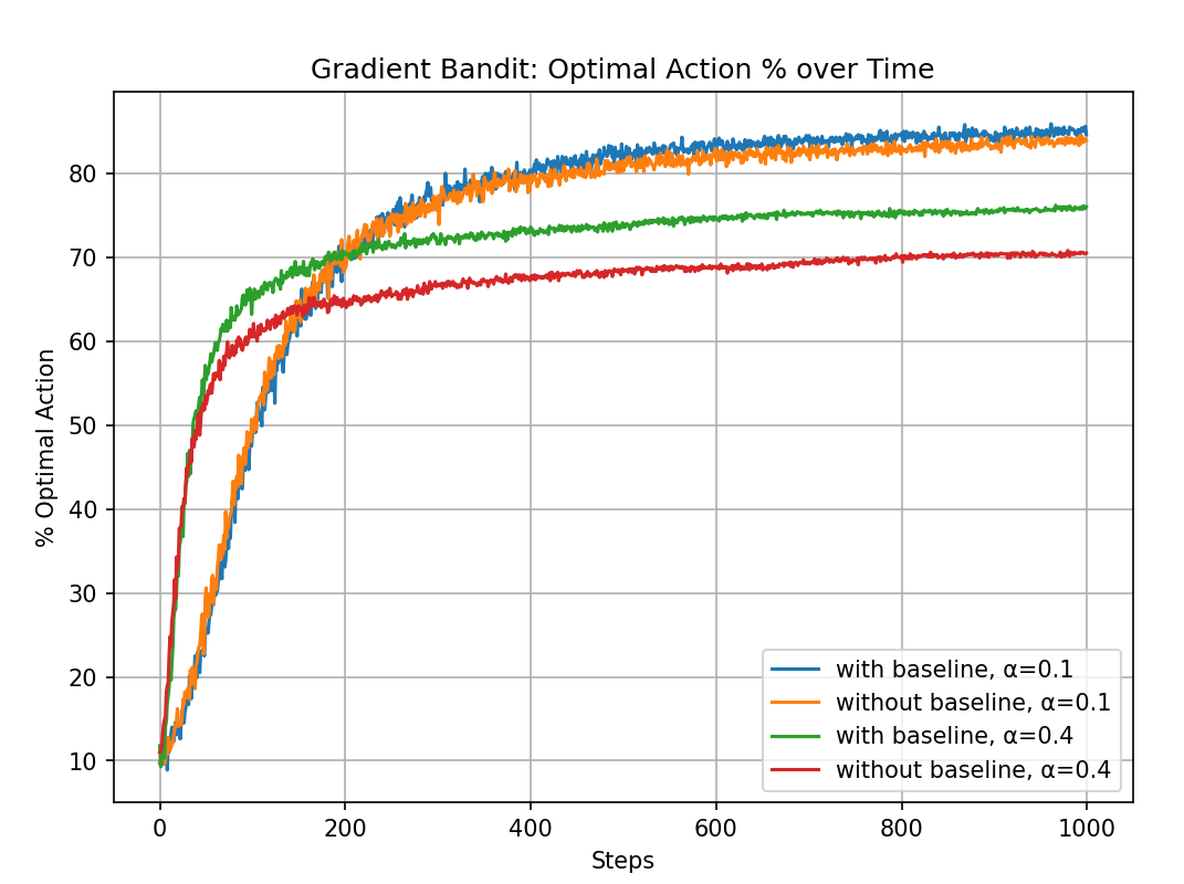
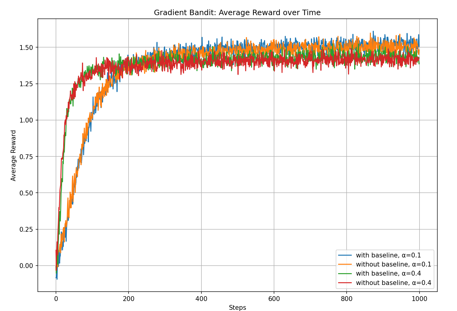
From the experimental results, we can see that the gradient bandit with a baseline outperforms the version without a baseline.
Note: The book inserts a deeper mathematical explanation of the gradient bandit algorithm here, showing that the algorithm is essentially performing stochastic gradient ascent on the expected reward. See Math 2.5: The Gradient Bandit Algorithm as Stochastic Gradient Ascent for details.
2.9 Associative Search (Contextual Bandits)
This section discusses Associative Search, also known as Contextual Bandits. In previous sections, we discussed only nonassociative tasks — tasks that do not require associating different situations with different actions. For example, the agent either searches for the single best action in a stationary task, or attempts to track the best action as it changes over time in a nonstationary task.
However, for more general reinforcement learning tasks, there is often more than one situation, and the learning objective includes context: finding a policy that can select the best action in each specific situation.
For example, suppose there are 3 machines that are identical except for color (say, red, green, and blue), each with 10 arms but different true reward distributions. If we ignore color and only consider the k-armed bandit problem itself, the agent cannot learn the correct policy. Therefore, the context (the color of the machine) must be incorporated into the learning objective. During learning, when the agent encounters the red machine, it can only choose among the red machine's arms and obtains the action-value function for the red machine. At this point, the value function includes the context, typically written as \(Q(s,a)\), where s represents the state — the "situation" we discuss here.
Exercise for this section: Exercise 2.10 from the book; see the appendix.
2.10 Chapter 2 Summary
In this chapter, we introduced several simple methods for balancing exploration and exploitation. Let us review and summarize the core formulas:
(1) Epsilon-greedy method
-
Probability of selecting the optimal action:
$$ P(a = a^*) = 1 - \varepsilon $$ - Probability of selecting a random action:
\[ P(a) = \frac{\varepsilon}{k}, \quad \text{for } a \ne a^* \]
(2) Optimistic initial values method
-
Initialization:
\[ Q_1(a) = Q_{\text{high}}, \quad \text{so that all actions appear highly valuable} \]
(3) UCB (Upper Confidence Bound) method
-
Action selection rule:
\[ A_t = \arg\max_a \left[ Q_t(a) + c \cdot \sqrt{\frac{\ln t}{N_t(a)}} \right] \]- \(Q_t(a)\): the current average reward of action \(a\)
- \(N_t(a)\): the number of times action \(a\) has been selected
- \(c\): a hyperparameter controlling the degree of exploration
(4) Gradient method (Gradient Bandit)
-
Uses the softmax distribution to select actions:
\[ P(a) = \frac{e^{H_t(a)}}{\sum_b e^{H_t(b)}} \]- \(H_t(a)\): action preference
- Preference update (using baseline \(\bar{R}_t\)):
The book provides the following figure showing the performance of these four methods on the multi-armed bandit problem:
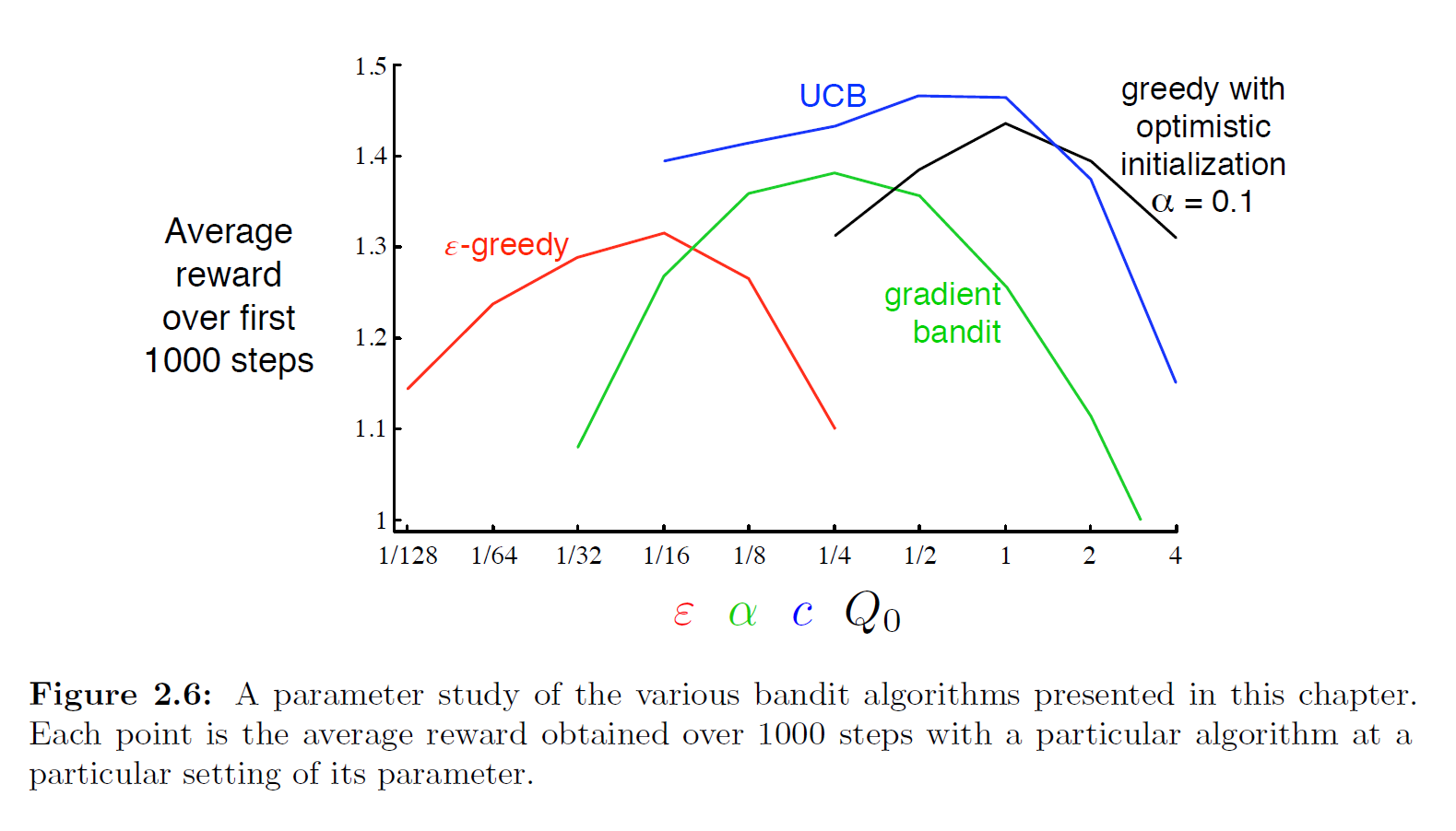
The author was too lazy to reproduce this figure here. The code for each method is in the Code appendix. Interested readers can try writing them all in a single file and plotting the comparison. From the figure provided in the book, UCB performs best among the four methods. The figure includes parameter variations, all using k=10 as the test environment, making the comparison fair. This type of comparison plot is called a parameter study, which compares the average performance of different algorithms under different parameter settings.
At the same time, when evaluating a method, we should not only look at its performance at the best parameter value, but also at its sensitivity to parameter changes. All four methods are relatively insensitive to parameter changes in this problem and exhibit stable performance. Algorithms that are insensitive to parameters are more robust, making them more suitable for practical applications, since tuning parameters in practice is difficult.
Although these four methods are sufficient for solving the k-armed bandit problem, we have not yet found a fully satisfactory solution for balancing exploration and exploitation. Another widely studied exploration-exploitation balancing method is the Gittins Index, which is a Bayesian method. Although the computational process of Bayesian methods is typically quite complex, for certain special distributions (called conjugate priors) the computation becomes simpler. One feasible approach is to use posterior sampling or Thompson sampling. Experiments show that this method performs comparably to or even better than all methods introduced in this chapter.
In a Bayesian setting, it is even possible to compute the optimal exploration-exploitation balance: for each possible action, you can compute the probability of obtaining an immediate reward and the probabilities of all future posterior distribution changes. These constantly changing distributions form the information state of the problem. However, in practice, this tree grows extremely fast and requires approximate methods for efficient computation — which amounts to converting the bandit problem into a full reinforcement learning problem. This topic is beyond the scope of this book. If the opportunity arises after completing a close reading of this book, the author may revisit these additional topics. (To be continued...)
Exercise for this section: Exercise 2.11 from the book; see the appendix.
Appendix: Exercises
Exercise 2.1 Computing the Greedy Action Selection Probability
Q: In ε-greedy action selection, suppose there are two actions and ε=0.5. What is the probability of selecting the greedy action?
A: If epsilon=0.5, then there is clearly a 0.5 probability of exploring and a 1-0.5=0.5 probability of selecting the greedy action. However, note that during random exploration, the greedy action may also be selected, so the total probability of the greedy action is generally computed as:
Exercise 2.2 Identifying ε-actions
Q:
Consider a k=4 multi-armed bandit problem with the following strategy:
- ε-greedy strategy
- Sample-average method for action-value estimation
- All initial action-value estimates set to \(Q_1(a)=0\) for all a
Suppose the actions taken and rewards received in the first few steps are:
| Timestep | Action | Reward |
|---|---|---|
| \(t=1\) | \(A_1=1\) | \(R_1=-1\) |
| \(t=2\) | \(A_2=2\) | \(R_2=1\) |
| \(t=3\) | \(A_3=2\) | \(R_3=-2\) |
| \(t=4\) | \(A_4=2\) | \(R_4=2\) |
| \(t=5\) | \(A_5=3\) | \(R_5=0\) |
At which time steps can we be certain that an ε-exploration occurred, and at which is it merely possible?
A:
| Timestep | Did ε occur? | Reason |
|---|---|---|
| 1 | Possible | At the first step all Q-values are 0, so ε or greedy makes no difference |
| 2 | Possible | At this point there are 4 equally optimal choices, so either case is possible |
| 3 | Possible | This step looks like greedy at first glance, but it could also be ε-exploration that randomly hit the optimal value |
| 4 | Certain | At this point a2 is no longer the optimal value, so selecting it must be due to ε |
| 5 | Certain | At this point a3's Q is 0, but a2's Q after three selections has been updated to 0.33, which is greater than a3's |
Exercise 2.3 Quantitative Expectations for Different ε Strategies
Q: For the comparison experiment shown in the figure, which method performs best in the long run? How much better is it? Can you express this quantitatively?
A: This is an interesting question that requires mathematical analysis. Although ε=0.1 clearly performs best in the figure, from a mathematical perspective, if we consider infinite time steps, i.e., \(t \to \infty\), then the sample-average estimate with exploration will converge to the true value for each action:
Let the arm with the highest true value be \(a^* = \arg\max_a q^*(a)\), and denote its true value as \(q^*_{\max} \;=\; q^*(a^*) \;=\; \max_{1 \le a \le 10} q^*(a)\). Under the ε-strategy, at each step:
- With probability 1-ε, \(a^*\) is selected
- With probability ε, a random arm is chosen from the 10, with probability ε/10 of selecting \(a^*\)
Therefore, as \(t\to\infty\) and \(Q_t\) is highly accurate, the probability of selecting the optimal arm \(a^*\) is:
In other words:
Similarly, the combined probability of selecting a non-optimal arm is:
Therefore, we can obtain the theoretical long-term average reward for a given epsilon value:
After mathematical transformation, we obtain the solvable long-term average reward (see Math 2.2 in the appendix for the derivation):
Therefore, we can quantitatively determine the theoretical long-term (limiting) probability of selecting the optimal arm, and the long-term (limiting) average reward:
| epsilon | \(P_\infty\) | \(\mathbb{E}[R_\infty]\) |
|---|---|---|
| 0 | N/A* | N/A* |
| 0.01 | 0.991 | (1-0.1)*1.54 |
| 0.1 | 0.91 | (1-0.01)*1.54 |
*Under greedy, the agent may get stuck on a suboptimal arm from the start; the idealized theoretical limit is 100%.
Exercise 2.4 Variable Step-Size Parameter Representation
Q: If the step-size parameter \(\alpha_n\) is not constant, the estimate \(Q_n\) is still a weighted average of previously received rewards, but with a different weighting scheme than the formula given in Section 2.5. In the more general case of variable step sizes, what is the weight of each previously received reward? Express these weights in terms of a sequence of step-size parameters, as a generalization of the formula in Section 2.5.
A: First, let us review the formula from Section 2.5 referenced in the problem: \(Q_n = (1 - \alpha)^n Q_0 + \sum_{i=1}^n \alpha (1 - \alpha)^{n - i} R_i\). This formula shows that Qn is actually an exponentially weighted moving average with decay.
If the step size \(\alpha_n\) is not constant, the estimate Qn is still a weighted average of all past rewards Ri, but the weight of each reward is determined by different step-size sequences:
The weight of the i-th reward Ri is:
This shows that each reward's weight depends not only on the step size \(\alpha_i\) at the time it was introduced, but also on the "decay effect" of all subsequent step sizes.
Note: For the derivation and explanation of this formula, see Math 2.3: Generalized Exponential Decay Weighted Average in the appendix.
Exercise 2.5 Nonstationary Experiment
Programming exercise: Design an experiment to demonstrate the difficulties that the sample-average method encounters on nonstationary problems. Specific requirements:
- The multi-armed bandit still has k=10
- Initialize all true action values \(q_*(a)\) to be equal
- At each step, apply independent random walks to all of them (e.g., add an increment drawn from a normal distribution with mean 0 and standard deviation 0.01 to each \(q_*(a)\) at every step)
- Use two different action-value methods: sample-average (incremental sample-average) and constant step-size (alpha=0.1)
- For both methods, under the same nonstationary environment, run a reasonably long simulation, e.g., 10,000 steps. Set epsilon=0.1 for ε-greedy.
- Plot the average reward curve (how the algorithm's average return changes as time steps progress) and the optimal action selection percentage curve (how frequently the algorithm selects the optimal action as time steps progress).
A:
Based on the requirements above, the pseudocode is as follows:
class 老虎机:
    def __init__():
        k = 10
        真实奖励q* = 长度为k的list,包含10个一样的值,可以都设置为0

    def 获得奖励(动作a):
        实际奖励 = 在以动作a的真实奖励为均值,方差为1的正态分布中采样
        对所有真实奖励q*永久性累加随机游走的扰动(均值为0、标准差为0.01)
        return 实际奖励

class Agent:
    def __init__():
        epsilon = 0.1
        Q数组,长度为10,初始化为0;存放每个动作当前的估计值
        N数组,长度为10,初始化为0;记录每个动作被选过的次数,用于样本平均法和统计使用

    def 动作选择():
        按照epsilon选择最优/随机动作

    def 更新Q值(更新方法, 动作a):
        N[动作a] += 1
        if 更新方法 = 样本平均法:
            按照样本平均法进行动作a的Q值更新
        else:
            按照固定步长法进行动作a的Q值更新,固定步长alpha=0.1

def main():
    分别模拟样本平均法和固定步长法:
        模拟2000次试验:
            在每次试验中进行100000个时间步:
                让Agent根据Q值选择动作
                获得奖励()
                更新Q值()
    完成后分别绘制平均奖励曲线和最优动作选择百分比曲线
    注:绘制曲线需要的额外变量并没有写在上述伪代码中
Send the above pseudocode to ChatGPT to generate Python code (see Code 2.2 Nonstationary Environment Experiment in the appendix). The results are as follows:
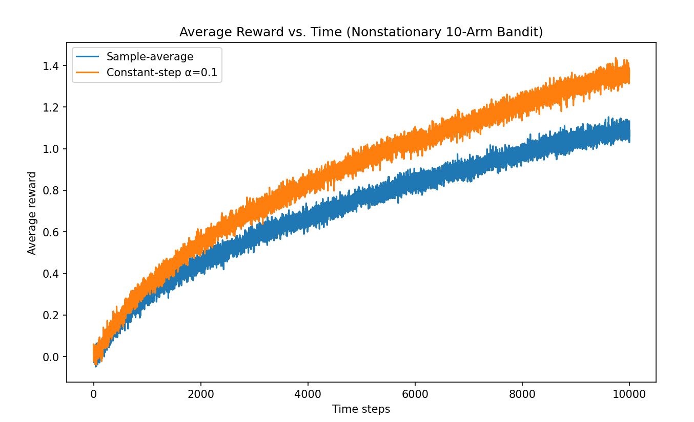
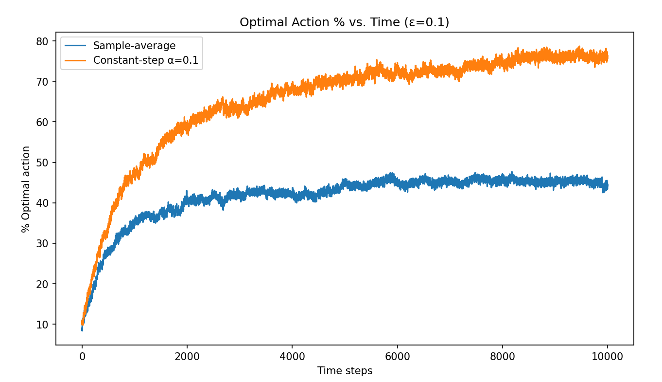
From the experimental results, the constant step-size method performs better in the nonstationary environment.
Exercise 2.6 Issues in the Optimistic Initial Values Figure
Q: In the optimistic initial values experiment in Section 2.6 (Code 2.3 Optimistic Initial Values), why do we see fluctuations and spikes early in the optimistic method's curve? In other words, what factors might cause this method to perform particularly well or particularly poorly at certain early steps on average?
A: In the optimistic initial values method, all initial estimated values are set very high (e.g., +5), while the actual rewards are sampled from a normal distribution with mean 0. Therefore, regardless of which action is chosen, the reward obtained the first time is almost always lower than the initial estimate, causing the Q-value to drop immediately.
This "disappointing" feedback causes the agent to quickly abandon the current action and try others. This is equivalent to almost fully exploratory behavior in the early stages — even without an explicit ε, every action gets tried in turn.
Why oscillations and spikes appear:
- Once a particular action happens to receive a reward above average, its Q-value drops more slowly or even temporarily rises, causing that action to be repeatedly selected for a few steps.
- But then, because the true reward is below the estimate, Q drops again, and the agent starts exploring other actions.
- During this process, a behavior of "suddenly favoring an action for a few steps and then abandoning it" occurs, leading to spikes and fluctuations in the average reward at these points.
Additionally, since the true rewards are randomly generated in each of the 2000 trials, these fluctuations are not fully averaged out in the first few dozen steps, which manifests as spikes in the early portion of the curve.
Exercise 2.7 Designing a Constant Step-Size Coefficient That Avoids Initial Bias
Q:
For most of this chapter, we used sample averages to estimate action values because sample averages do not produce the initial bias that constant step sizes do. However, sample averages are not entirely satisfactory because they may perform poorly on nonstationary problems.
Is it possible to retain the advantages of constant step sizes for nonstationary problems while avoiding their initial bias? One approach is to use the following step size:
for the n-th reward of a particular action, where \(\alpha > 0\) is a conventional constant step size and \(\bar{o}_n\) is a "trace of one" starting from 0, defined as:
Prove that using this method, the resulting Qn is an exponentially weighted average with no initial bias.
A:
From the recurrence, we obtain:
Therefore \(\beta_1 = \alpha / \alpha = 1\). The first update yields ( Q_1 = R_1 ), completely erasing ( Q_0 ) (no initial bias). Recursively expanding \(Q_n = Q_{n-1} + \beta_n (R_n - Q_{n-1})\), we get:
Let the coefficients be:
We can observe that:
Since \(\alpha\) is a predetermined constant satisfying \(0<\alpha<1\), the above holds. This means that for fixed n, \(w_i^{(n)}\) increases geometrically with i, or equivalently, decays backward in time at a rate of \((1-\alpha)\). That is, \(w_i^{(n)}\) forms typical "exponentially decaying and normalized" weights. Therefore ( Q_n ) is indeed an exponentially weighted average with no initial bias.
For the detailed explanation, see Math 2.4: Designing Unbiased Constant Step-Size Update with Exponentially Weighted Average Coefficients.
Exercise 2.8 UCB Spike
Q: In Figure 2.4 from the book (shown below), UCB exhibits a noticeable spike at step 11. Explain why this spike appears and why it drops rapidly afterward. Hint: if c=1, the spike would not be as pronounced.
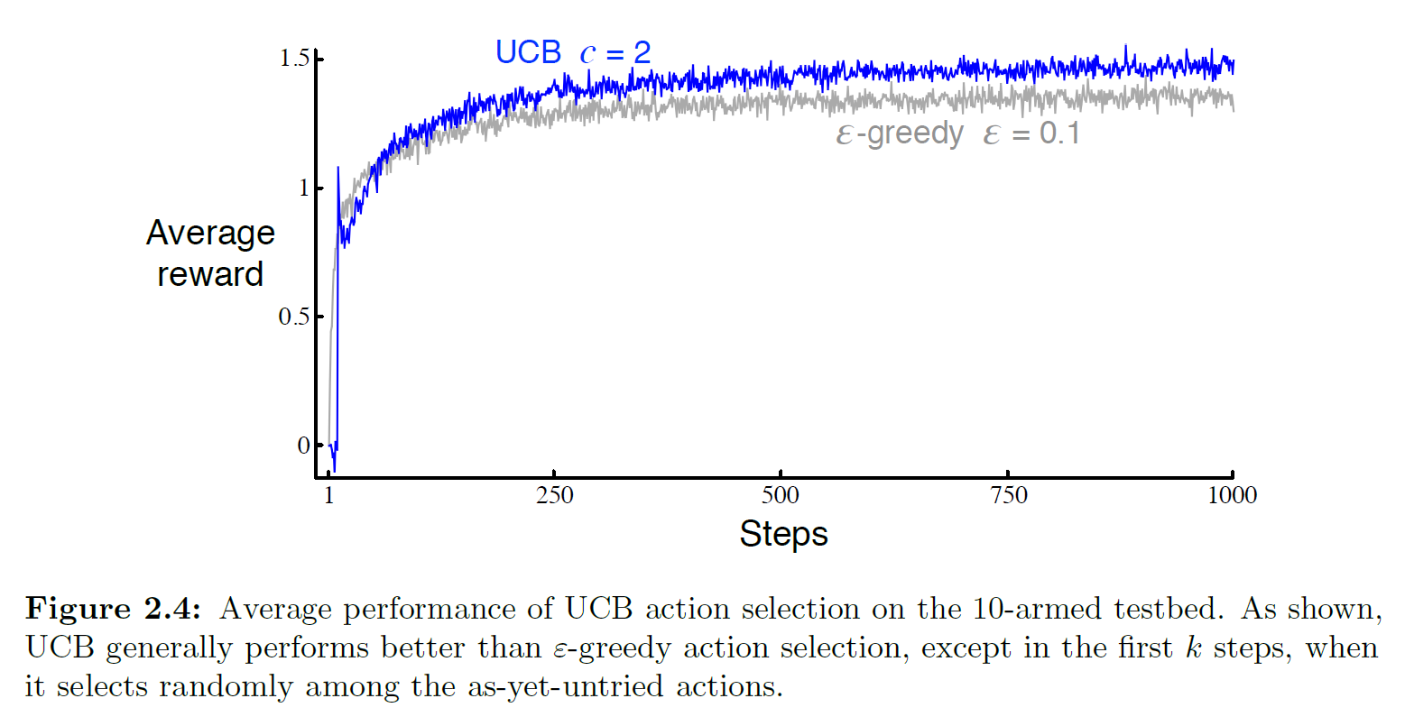
A: Since k=10, according to the UCB formula, the first 10 steps effectively try each action once. At step 11, since every action has been tried once, they all have Nt(a) = 1, so the exploration bonus is the same for all arms: \(c \sqrt{\frac{\ln(11)}{1}}\). Therefore, step 11 will necessarily select the arm that happened to have the highest initial sample, but once that arm is selected, its Nt(a) increases, causing its exploration bonus to decrease. This leads to a brief drop in reward until the overall exploration bonus exceeds the UCB values of other arms, at which point it is selected again and continues to be selected.
It is worth noting that as t grows, we can consider Nt(a) = O(t), so as t increases, the exploration bonus ultimately approaches 0. In other words, when t is large, the exploration bonus term becomes nearly negligible, causing the UCB strategy to become an approximately greedy strategy.
As for why the spike is smaller when c=1: c acts as the coefficient of the exploration bonus, so reducing c reduces the bonus overall.
Exercise 2.9 Mathematical Proof
Prove: The soft-max distribution in the case of only two actions is equivalent to the logistic function (or sigmoid function) commonly used in statistics and neural networks.
A: Let the two actions be 0 and 1. Then:
where \(x = H_t(1) - H_t(0)\) represents the relative preference of action 1 over action 0.
Exercise 2.10 Contextual Bandit Task
Q:
Suppose you face a two-armed bandit task in which the true action values change randomly from step to step. Specifically, suppose that at any time step, the true values of actions 1 and 2 are either 10 and 20 (Case A, with probability 0.5) or 90 and 80 (Case B, with probability 0.5).
- If you cannot distinguish which case you are in at any time, what is the best expected reward you can achieve? How should you choose actions to achieve this?
- Now suppose at each time step, you are told whether you are in Case A or Case B (though you still do not know the exact true values of the actions). This is an associative search task. In this case, what is the best expected reward you can achieve? How should you choose actions to achieve it?
A:
Assume the problem describes a standard stationary problem.
For the first question, if the cases cannot be distinguished, we can compute the expected value of each action and find that both action 1 and action 2 have a total expected value of 50. Therefore, regardless of the strategy, the optimal expected reward is the same — always selecting action 1, always selecting action 2, or selecting each with 50% probability at each step are all optimal.
For the second question, we can set up Q(s,a) to record the four cases:
| True values of actions 1 and 2 | Action 1 | Action 2 |
|---|---|---|
| Case A: with probability 0.5 | Q(A,1)=10 | Q(A,2)=20 |
| Case B: with probability 0.5 | Q(B,1)=90 | Q(B,2)=80 |
In this case, it is easy to compute the optimal expected reward as \(0.5 \times 20 + 0.5 \times 90 = 55\). Without knowing the true values, following the Q(s,a) setup above, we simply add observation of the case when observing, and make sure to record correctly. Everything else is the same as what we have already learned.
Exercise 2.11 Parameter Study for the Nonstationary Setting
Programming exercise: For the nonstationary setting described in Exercise 2.5, plot a parameter study. Requirements:
- Include the ε-greedy algorithm with constant step size, where \(α = 0.1\).
- Each experiment runs for 200,000 steps.
- The performance metric for each algorithm and parameter setting should be the average reward over the last 100,000 steps.
A:
See Code 2.6 for the detailed code. The author used ChatGPT to write a GPU-accelerated version, since the standard version would have taken about 10 hours to run. Results are as follows:
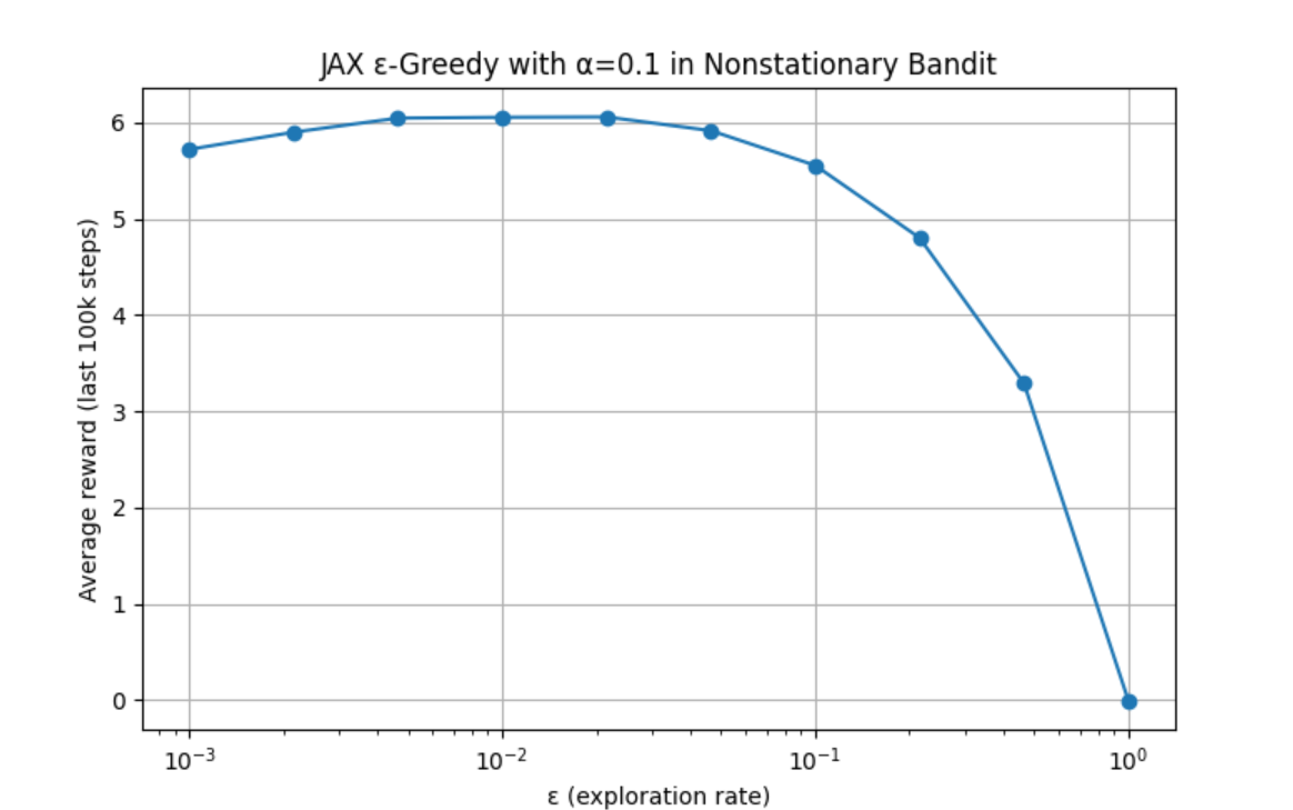
Increasing the number of sample points to 100 yields:
Appendix: Math
Math 2.1 Proving the Theoretical Optimal Expected Reward for the Multi-armed Bandit Experiment
It can be mathematically proved that the theoretical optimal value for the multi-armed bandit problem is 1.54.
(Note: This proof was derived by the author by looking up references while reading the book. If there are any errors, please contact the author to prevent misleading others.)
In our setup, the 10 true rewards follow a standard normal distribution. What we need to find is the expected value of the maximum of 10 independent standard normal random variables. Since the actual reward fluctuates around the true reward with a standard normal distribution (noise with mean 0), in the infinitely long run, the corresponding average reward necessarily converges to the true value.
Therefore, the theoretical optimal value is the expected maximum of 10 standard normal random variables.
For k independent standard normal random variables:
Their maximum Mk is:
In statistics, \(\{ X_{(1)}, X_{(2)}, \ldots, X_{(k)} \}\) are called the Order Statistics of this sample, where \(X_{(1)} \le X_{(2)} \le \cdots \le X_{(k)}\). Then \(X_{(k)} = M_k = \max\{X_1, \ldots, X_k\}\).
Using the distribution and expectation formula for the maximum order statistic, we first obtain the cumulative distribution function (CDF):
Then differentiating to get the probability density function (PDF):
The expected maximum is then:
Substituting k=10:
That is, when k=10, the mathematical expectation of the maximum among 10 slot machines is:
Math 2.2 Deriving the Solvable Theoretical Average Optimal Reward for Multi-armed Bandits
Below is a derivation that was not fully expanded in Exercise 2.3.
In Exercise 2.3, through a simple derivation, we obtain the long-term average reward with 10 actions and optimal arm \(a^*\):
Examining the coefficient in the left part of (1), we split it:
Substituting back into (1), we get (2):
where:
- A is the expected value from the greedy phase directly selecting the optimal arm
- B is the expected value from the exploration phase happening to select the optimal arm
- C is the expected value from the exploration phase selecting any non-optimal arm
Next, we merge (B) and (C) from (2) to get the exploration phase contribution from all 10 arms. This requires a small trick. First, write out the decomposition of "the sum of values over all 10 arms":
Then multiply both sides of (I) by ε/10:
(II) is equivalent to:
Substituting (III) back into (2), we get (3):
In equation (3), \(q^*_{\text{max}}\) on the left is the \(\mathbb{E}\left[ \max_{1 \le i \le 10} q_i^* \right]\) derived in Math 2.1. When k=10:
For the right part, for 10 values set up as i.i.d. (independent and identically distributed) standard normal variables, the expectation of their sum is 0:
Therefore, for the entire equation (3), under k=10 with a standard normal distribution environment, it is equivalent to:
Math 2.3 Generalized Exponential Decay Weighted Average
First, we start from the basic update formula:
Rearranging into "linear weighting" form:
This form tells us that the current estimate Qn is partially retained (by a factor of \(1-\alpha_n\)), and the new reward Rn is added with weight \(\alpha_n\). We can similarly write the linear weighting form for Qn:
Substituting (2) into (1):
Repeating this expansion produces a "nested" structure:
We can then observe that when i=n, the corresponding term in the sum is:
In mathematics, when the lower bound of a product exceeds the upper bound, it is called an empty product, and by convention its value is 1:
Therefore, when \(i=n\), the last term \(\alpha_nR_n\) is actually the i=n term in the summation. This repeating pattern can be expressed as:
In simple terms:
Math 2.4 Designing Unbiased Constant Step-Size Update with Exponentially Weighted Average Coefficients
1. Design Idea: How to Construct Unbiased Constant Step-Size Update Coefficients
In the common constant step-size update, we typically use
but this leaves a residual "initial bias" from \(Q_0\) — because expanding gives
where \((1-\alpha)^n Q_0\) never fully disappears. If we want to simultaneously achieve:
- No dependence on \(Q_0\) from step 1 onward (no initial bias),
- Continued fast response to new data (approximate constant step-size \(\alpha\) effect) for subsequent steps,
then we need step 1 to use step size 1 (completely erase \(Q_0\)), while at step \(n>1\) "gradually returning to" the constant \(\alpha\).
1.1 Constructing the auxiliary sequence \(\bar o_n\)
We first define an auxiliary variable sequence \(\{\bar o_n\}\) for dynamically "normalizing" the constant \(\alpha\):
-
Let
$$ \bar o_0 = 0; $$ - For \(n \ge 1\), the recurrence is
\[ \bar o_n \;=\; \bar o_{n-1} + \alpha\,\bigl(1 - \bar o_{n-1}\bigr). \]In short, \(\bar o_n\) starts at 0 and "approaches 1 by a small step" at each iteration, with the rate determined by \(\alpha\).
1.2 Defining the dynamic step size \(\beta_n\)
Based on \(\bar o_n\), we define the step size for the n-th update as
This gives:
-
Step 1: \(\bar o_1 = \alpha\), so
\[ \beta_1 = \frac{\alpha}{\alpha} = 1. \]Using \(\beta_1=1\) at step 1 yields
\[ Q_1 = Q_0 + 1\cdot\bigl(R_1 - Q_0\bigr) = R_1, \]thereby completely erasing the initial \(Q_0\) and ensuring "no initial bias." - Step \(n>1\): \(\bar o_n \to 1\), therefore
\[ \beta_n = \frac{\alpha}{\,\bar o_n\,} \;\approx\; \alpha\quad(\text{when }n\text{ is sufficiently large})\,. \]The step size \(\beta_n\) for subsequent updates rapidly decreases from 1 to approximately \(\alpha\), thus recovering the constant step-size effect and maintaining fast response to new data.
In summary, the design result:
- Step 1: \(\beta_1=1\) -> immediately erases \(Q_0\) -> no initial bias;
- Step \(n>1\): \(\beta_n=\alpha/\bar o_n\) -> as \(\bar o_n\to1\), rapidly approaches \(\alpha\) -> retains the advantages of constant step size.
2. Detailed Proof: These Coefficients Are Unbiased and Form an Exponentially Weighted Average
Below, given the definitions of \(\bar o_n\) and \(\beta_n\), we prove the required properties step by step. Proving no initial bias shows that the artificial initial value can be eliminated; proving normalization shows that these weights form a true weighted average — the influence of historical rewards both decays exponentially and has total weight equal to 1, without being artificially amplified or diminished.
2.1 Deriving the Closed-form Expression for \(\bar o_n\)
First, we prove that the recurrence
is equivalent to
Verification (mathematical induction):
- When \(n=0\): \(1 - (1-\alpha)^0 = 0 = \bar o_0\).
- Assume for some \(n-1\ge0\) it holds: \(\bar o_{n-1} = 1 - (1-\alpha)^{\,n-1}\).
- Then:
Induction complete.
Therefore
In particular, when \(n=1\), \(\beta_1 = \alpha/\alpha = 1\).
2.2 Step 1 Erases \(Q_0\): Verifying No Initial Bias
The update formula is
-
Step 1: \(\beta_1=1\), so
\[ Q_1 = Q_0 + 1\,(R_1 - Q_0) = R_1, \]completely removing the dependence on \(Q_0\). - Recursive expansion: for any \(n\ge1\), applying the update formula gives
Since \(\beta_1=1\implies(1-\beta_1)=0\), we have \(C_0^{(n)}=0\), so \(Q_n\) does not contain \(Q_0\). Let
then
This demonstrates "no initial bias whatsoever."
2.3 Deriving Exponential Decay and Normalization
-
Computing \(1-\beta_j\):
$$ \beta_j = \frac{\alpha}{\,1 - (1-\alpha)^j\,} \;\implies\; 1 - \beta_j = \frac{(1-\alpha)\,\bigl[\,1 - (1-\alpha)^{\,j-1}\bigr]}{\,1 - (1-\alpha)^j\,}. $$ 2. Taking the product and canceling intermediate factors:
$$ \prod_{j=i+1}^n (1 - \beta_j) = \prod_{j=i+1}^n \frac{(1-\alpha)\,[\,1 - (1-\alpha)^{\,j-1}\,]}{\,1 - (1-\alpha)^j\,} = \frac{(1-\alpha)^{\,n - i}}{\,1 - (1-\alpha)^n\,}. $$ 3. Obtaining the simplified form of \(w_i^{(n)}\):
$$ w_i^{(n)} = \beta_i \prod_{j=i+1}^n (1 - \beta_j) = \frac{\alpha}{\,1 - (1-\alpha)^i\,} \;\times\;\frac{(1-\alpha)^{\,n - i}}{\,1 - (1-\alpha)^n\,} = \frac{\alpha\,(1-\alpha)^{\,n - i}}{\,1 - (1-\alpha)^n\,}. $$ 4. Verifying normalization:
$$ \sum_{i=1}^n w_i^{(n)} = \sum_{i=1}^n \frac{\alpha\,(1-\alpha)^{\,n - i}}{\,1 - (1-\alpha)^n\,} = \frac{1}{\,1 - (1-\alpha)^n\,} \sum_{i=1}^n \alpha\,(1-\alpha)^{\,n - i} = 1. $$
Therefore
is both exponentially decaying and normalized as a weighted average.
Summary: The above proves that the designed \(\beta_n=\alpha/\bar o_n\) both ensures no initial bias (\(\beta_1=1\) erases \(Q_0\)) and yields
so that \(Q_n\) is an exponentially weighted average with no initial bias.
This "unbiased constant step-size + exponential weighting" design technique is a classic scheme in reinforcement learning. On one hand, it erases the initial value (the artificially specified Q0 in algorithm design) so that the first estimate comes directly from real data rather than an artificial setting; on the other hand, it retains the constant step-size advantage of rapid response to new information.
Math 2.5 The Gradient Bandit Algorithm as Stochastic Gradient Ascent
We can gain deeper insight into the gradient bandit algorithm by understanding it as a stochastic approximation to gradient ascent.
In exact gradient ascent, each action preference \(H_t(a)\) is updated incrementally in proportion to the effect of that preference on performance:
where the "performance" being measured is the expected reward:
- Here \(\pi_t(x)\) is the probability of selecting action \(x\) at time \(t\);
- \(q_*(x)\) is the true mean return of action \(x\) (but in practice we do not know \(q_*(x)\)).
The effect of the increment on performance is the partial derivative of this "performance measure" with respect to the action preference \(H_t(a)\). Of course, in our multi-armed bandit setting, we cannot exactly perform this "exact gradient ascent" because we do not know \(q_*(x)\) for any action. However, our algorithm's update rule is in fact equivalent to the above equation (3) in expectation, making the algorithm a form of stochastic gradient ascent. Completing this proof requires only elementary calculus, though the steps are somewhat lengthy. Below we start with the proof of the Soft-max partial derivative, then return to the stochastic update derivation.
I. Computing \(\displaystyle \frac{\partial\,\pi_t(x)}{\partial\,H_t(a)}\)
Consider the Soft-max policy
Let the numerator be \(f(x)=e^{H_t(x)}\) and the denominator be \(g=\sum_{y=1}^k e^{H_t(y)}\). We want to compute
- Applying the quotient rule
- Computing \(\displaystyle \frac{\partial\,f(x)}{\partial\,H_t(a)}\)
- Computing \(\displaystyle \frac{\partial\,g}{\partial\,H_t(a)}\)
- Substituting the above results into the quotient rule. The two terms in the numerator are
Therefore
- Extracting common factors and simplifying the numerator. Split the numerator into two parts:
Note that
Therefore
The final result is
This completes the proof of the partial derivative of the Soft-max policy from equation (1):
II. Deriving the Exact Performance Gradient
First, write the performance gradient with respect to an action preference \(H_t(a)\):
Since \(q_*(x)\) is independent of \(H_t(a)\), we can interchange the sum and derivative, applying the derivative to \(\pi_t(x)\):
Next, introduce a baseline \(B_t\). As long as this baseline is a scalar independent of action \(x\), adding or subtracting it does not change the gradient, because
since \(\sum_x \pi_t(x) = 1\) always holds; when taking the partial derivative with respect to \(H_t(a)\), the increments of the individual \(\pi_t(x)\) cancel out, summing to zero.
Thus we can subtract \(B_t\) in the original expression without changing the result:
Here \(B_t\) is called a baseline; as long as it does not depend on action \(x\), it does not affect the total gradient.
III. Writing the Gradient in Expectation Form
To express the above as an expectation, multiply each term by \(\displaystyle \frac{\pi_t(x)}{\pi_t(x)}\), allowing us to write it as an expectation over the random variable \(A_t\):
This way, the right side is an expectation over "the random variable \(A_t\) representing which action is selected at time \(t\)":
When sampling, the immediate reward \(R_t\) we obtain is drawn from the "true distribution of action \(x\)," so \(q_*(A_t)\) can be replaced by the unbiased estimate \(R_t\), and \(B_t\) can be approximated by the cumulative average reward \(\bar{R}_t\) (in fact, any scalar independent of \(A_t\) works). This gives:
At this point, the "performance gradient" is written in expectation form — the expected value of "a single sample's contribution to the gradient."
IV. Stochastic Gradient Ascent Sample Update
Recall our original goal: to write the performance gradient (from equation (3): \(\displaystyle \frac{\partial\,\mathbb{E}[R_t]}{\partial\,H_t(a)}\)) as an expression that can be sampled at each step, then use that sample to make incremental updates to preferences. Following the derivation above, if we approximate the expectation with a single random sample, we get:
Combining with the result proved in Part I:
we obtain the familiar gradient bandit update formula (equation (2)):
where \(\mathbb{1}_{\,a = A_t}\) is the indicator: 1 if \(a\) equals the selected action \(A_t\), and 0 otherwise. This completes the derivation of the gradient bandit algorithm's update rule within the stochastic gradient ascent framework.
We have thus shown that the gradient bandit algorithm's update is equivalent in expectation to performing gradient ascent on the "expected reward," making it an instance of stochastic gradient ascent with good convergence properties.
It is important to note that the only requirement on the "baseline (\(B_t\))" in the above derivation is that it does not depend on the selected action. For example, even setting \(B_t\) to 0 or to some constant like 1000 would not change the form of the "expected update," because \(\displaystyle \sum_x \frac{\partial\,\pi_t(x)}{\partial\,H_t(a)} = 0\). The choice of baseline does not affect the expected update but does affect the variance of the update, which in turn affects convergence speed (as shown in Figure 2.5). In practice, we typically set the baseline to the running average of all rewards up to the current time, which is both simple and performs well.
Appendix: Code
Code 2.1 Multi-armed Bandit Experiment
import numpy as np
import matplotlib.pyplot as plt
from tqdm import tqdm

# ----------------------------
# 类:多臂老虎机环境(BanditEnv)
# ----------------------------
class BanditEnv:
    def __init__(self, k=10):
        self.k = k
        # 按照标准正态分布生成 k 个动作的真实平均奖励 q*
        self.q_star = np.random.normal(0, 1, k)
        # 记录当前环境下的最优动作索引
        self.best_action = np.argmax(self.q_star)

    def get_reward(self, action):
        """
        根据动作 a 的真实平均值 self.q_star[action],从 N(q_star[action], 1) 中采样
        并返回该次的奖励
        """
        return np.random.normal(self.q_star[action], 1)


# ----------------------------
# 类:ε-Greedy 智能体(EpsilonGreedyAgent)
# ----------------------------
class EpsilonGreedyAgent:
    def __init__(self, k, epsilon):
        # 探索概率 ε
        self.epsilon = epsilon
        self.k = k
        # 初始化 k 个动作的估计值 Q[a] = 0
        self.Q = np.zeros(k)
        # 初始化每个动作被选择的计数 N[a] = 0
        self.N = np.zeros(k)

    def select_action(self):
        """
        ε-greedy 策略:
        - 以 ε 的概率随机探索动作;
        - 否则以 1−ε 的概率进行贪心选择(选择当前 Q[a] 最大的动作,若有并列则随机选一个)。
        """
        if np.random.rand() < self.epsilon:
            return np.random.randint(0, self.k)
        else:
            max_Q = np.max(self.Q)
            candidates = np.where(self.Q == max_Q)[0]
            return np.random.choice(candidates)

    def update(self, action, reward):
        """
        样本平均法更新 Q 值:
            N[a] += 1
            Q[a] ← Q[a] + (1 / N[a]) * (reward − Q[a])
        """
        self.N[action] += 1
        self.Q[action] += (reward - self.Q[action]) / self.N[action]


# ----------------------------
# 函数:run_one_episode
#   执行一次(单 trial)→ 固定 k, steps, ε
# ----------------------------
def run_one_episode(k, steps, epsilon):
    """
    对应于单次试验(1000 步):
    - 先初始化 环境(BanditEnv) 和 智能体(EpsilonGreedyAgent);
    - 每个时间步 t:
        1. agent.select_action() 选择动作 a
        2. reward = env.get_reward(a)
        3. agent.update(a, reward)
        4. 记录 rewards[t] 和 是否选到最优动作 optimal_actions[t]
    返回:
      rewards:           长度为 steps 的奖励序列
      optimal_actions:   长度为 steps 的二值序列(1 表示该步选到最优动作)
    """
    env = BanditEnv(k)
    agent = EpsilonGreedyAgent(k, epsilon)
    rewards = np.zeros(steps)
    optimal_actions = np.zeros(steps)

    for t in range(steps):
        a = agent.select_action()
        r = env.get_reward(a)
        agent.update(a, r)

        rewards[t] = r
        if a == env.best_action:
            optimal_actions[t] = 1

    return rewards, optimal_actions


# ----------------------------
# 函数:run_experiment
#   对不同 ε 值,进行多次 runs(例如 2000 次)试验,统计平均
#   同时在 runs 循环中使用 tqdm 显示进度
# ----------------------------
def run_experiment(k=10, steps=1000, runs=2000, epsilons=[0, 0.01, 0.1]):
    """
    输出:
      avg_rewards:      形状为 (len(epsilons), steps) 的数组,每行对应某个 ε 的"每步平均奖励"
      optimal_rates:    形状为 (len(epsilons), steps) 的数组,每行对应某个 ε 的"每步最优动作命中率(%)"
    """
    avg_rewards = np.zeros((len(epsilons), steps))
    optimal_rates = np.zeros((len(epsilons), steps))

    for idx, epsilon in enumerate(epsilons):
        # tqdm 显示当前 ε 下的 runs 次试验进度
        for _ in tqdm(range(runs), desc=f"ε = {epsilon}"):
            rewards, optimal_actions = run_one_episode(k, steps, epsilon)
            avg_rewards[idx] += rewards
            optimal_rates[idx] += optimal_actions

        # 对 runs 次试验结果求平均
        avg_rewards[idx] /= runs
        # 由命中次数转换为百分比
        optimal_rates[idx] = (optimal_rates[idx] / runs) * 100

    return avg_rewards, optimal_rates


# ----------------------------
# 主程序入口
# ----------------------------
if __name__ == "__main__":
    # 参数设定
    k = 10
    steps = 1000
    runs = 2000
    epsilons = [0, 0.01, 0.1]

    # 运行实验,显示进度条
    avg_rewards, optimal_rates = run_experiment(k, steps, runs, epsilons)

    # 可视化:不同 ε 下的平均奖励曲线
    plt.figure(figsize=(12, 5))
    for idx, epsilon in enumerate(epsilons):
        plt.plot(avg_rewards[idx], label=f"ε = {epsilon}")
    plt.xlabel("Time Step")
    plt.ylabel("Average Reward")
    plt.legend()
    plt.title("Average Reward over Time for Different ε Values")
    plt.grid(True)
    plt.show()

    # 可视化:不同 ε 下的最优动作选择率(百分比)曲线
    plt.figure(figsize=(12, 5))
    for idx, epsilon in enumerate(epsilons):
        plt.plot(optimal_rates[idx], label=f"ε = {epsilon}")
    plt.xlabel("Time Step")
    plt.ylabel("Optimal Action Percentage (%)")
    plt.legend()
    plt.title("Percentage of Optimal Action over Time for Different ε Values")
    plt.grid(True)
    plt.show()
Code 2.2 Nonstationary Experiment
import numpy as np
import matplotlib.pyplot as plt
from tqdm import tqdm  # Import tqdm for progress bars

class NonstationaryBandit:
    def __init__(self, k=10, q_init=0.0, random_walk_std=0.01):
        self.k = k
        self.q_true = np.ones(k) * q_init
        self.random_walk_std = random_walk_std

    def get_reward(self, action):
        # Sample reward from N(q_true[action], 1)
        reward = np.random.normal(loc=self.q_true[action], scale=1.0)
        # Apply random walk to q_true for all actions
        self.q_true += np.random.normal(loc=0.0, scale=self.random_walk_std, size=self.k)
        return reward

    def optimal_action(self):
        return np.argmax(self.q_true)

class Agent:
    def __init__(self, k=10, epsilon=0.1, alpha=None):
        self.k = k
        self.epsilon = epsilon
        self.alpha = alpha  # None for sample-average, otherwise fixed-step size
        self.Q = np.zeros(k)
        self.N = np.zeros(k, dtype=int)

    def select_action(self):
        if np.random.rand() < self.epsilon:
            return np.random.randint(self.k)
        else:
            max_val = np.max(self.Q)
            candidates = np.where(self.Q == max_val)[0]
            return np.random.choice(candidates)

    def update(self, action, reward):
        self.N[action] += 1
        if self.alpha is None:
            n = self.N[action]
            self.Q[action] += (1.0 / n) * (reward - self.Q[action])
        else:
            self.Q[action] += self.alpha * (reward - self.Q[action])

def run_experiment(n_runs=2000, n_steps=10000, epsilon=0.1, alpha=None):
    avg_rewards = np.zeros(n_steps)
    optimal_action_counts = np.zeros(n_steps)

    # Use tqdm to display progress over runs
    for _ in tqdm(range(n_runs), desc=f'Running {"Sample-Average" if alpha is None else "Constant-Step α="+str(alpha)}'):
        env = NonstationaryBandit()
        agent = Agent(epsilon=epsilon, alpha=alpha)

        for t in range(n_steps):
            action = agent.select_action()
            reward = env.get_reward(action)
            agent.update(action, reward)

            avg_rewards[t] += reward
            if action == env.optimal_action():
                optimal_action_counts[t] += 1

    avg_rewards /= n_runs
    optimal_action_percents = (optimal_action_counts / n_runs) * 100.0
    return avg_rewards, optimal_action_percents

# Parameters
n_runs = 2000
n_steps = 10000  # Reduced from 100000 for reasonable output
epsilon = 0.1

# Run and plot for Sample-Average method
avg_rewards_sample, opt_percents_sample = run_experiment(
    n_runs=n_runs, n_steps=n_steps, epsilon=epsilon, alpha=None
)

# Run and plot for Constant-Step method (alpha = 0.1)
avg_rewards_const, opt_percents_const = run_experiment(
    n_runs=n_runs, n_steps=n_steps, epsilon=epsilon, alpha=0.1
)

# Plot average rewards
plt.figure(figsize=(10, 4))
plt.plot(avg_rewards_sample, label="Sample-average")
plt.plot(avg_rewards_const, label="Constant-step α=0.1")
plt.xlabel("Time steps")
plt.ylabel("Average reward")
plt.legend()
plt.title("Average Reward vs. Time (Nonstationary 10-Arm Bandit)")
plt.show()

# Plot % optimal action
plt.figure(figsize=(10, 4))
plt.plot(opt_percents_sample, label="Sample-average")
plt.plot(opt_percents_const, label="Constant-step α=0.1")
plt.xlabel("Time steps")
plt.ylabel("% Optimal action")
plt.legend()
plt.title("Optimal Action % vs. Time (ε=0.1)")
plt.show()
Code 2.3 Optimistic Initial Values
import numpy as np
import matplotlib.pyplot as plt

# 老虎机环境
class SlotMachine:
    def __init__(self, k=10):
        self.k = k
        self.real_q = np.random.normal(0, 1, k)  # 每个动作的真实期望奖励

    def reward(self, a):
        return np.random.normal(self.real_q[a], 1)  # 奖励分布 N(real_q[a], 1)

# 代理
class Agent:
    def __init__(self, Q_init, epsilon, alpha=0.1, k=10):
        self.Q = np.ones(k) * Q_init  # 初始化 Q 表
        self.epsilon = epsilon        # ε-贪婪参数
        self.alpha = alpha            # 学习率
        self.k = k

    def choose_action(self):
        if np.random.rand() < self.epsilon:
            return np.random.randint(0, self.k)  # 探索
        else:
            return np.argmax(self.Q)             # 利用

    def update_Q(self, a, reward):
        self.Q[a] += self.alpha * (reward - self.Q[a])  # Q 更新公式

# 主实验函数
def main(runs=2000, steps=1000):
    avg_rewards_1 = np.zeros(steps)  # 乐观初始值策略
    avg_rewards_2 = np.zeros(steps)  # ε-贪婪策略

    for run in range(runs):
        bandit = SlotMachine()
        agent1 = Agent(Q_init=5, epsilon=0)        # 乐观贪婪
        agent2 = Agent(Q_init=0, epsilon=0.1)      # ε-贪婪

        rewards1 = []
        rewards2 = []

        for t in range(steps):
            # Agent 1
            a1 = agent1.choose_action()
            r1 = bandit.reward(a1)
            agent1.update_Q(a1, r1)
            rewards1.append(r1)

            # Agent 2
            a2 = agent2.choose_action()
            r2 = bandit.reward(a2)
            agent2.update_Q(a2, r2)
            rewards2.append(r2)

        avg_rewards_1 += np.array(rewards1)
        avg_rewards_2 += np.array(rewards2)

    # 求平均
    avg_rewards_1 /= runs
    avg_rewards_2 /= runs

    # 绘图
    plt.figure(figsize=(10, 6))
    plt.plot(avg_rewards_1, label='Optimistic Greedy Q=5, ε=0')
    plt.plot(avg_rewards_2, label='ε-Greedy Q=0, ε=0.1')
    plt.xlabel("Steps")
    plt.ylabel("Average Reward")
    plt.title("Optimistic Initial Values vs ε-Greedy")
    plt.legend()
    plt.grid(True)
    plt.show()

# 运行实验
if __name__ == "__main__":
    main()
Code 2.4 UCB
import numpy as np
import matplotlib.pyplot as plt

np.random.seed(42)

class Bandit:
    def __init__(self, k=10):
        self.k = k
        self.real_q = np.random.normal(0, 1, k)

    def reward(self, a):
        return np.random.normal(self.real_q[a], 1)


class AgentUCB:
    def __init__(self, k=10, c=2):
        self.k = k
        self.c = c
        self.Q = np.zeros(k)
        self.counts = np.zeros(k, dtype=int)
        self.total_count = 0

    def choose_action(self):
        self.total_count += 1
        ucb_values = self.Q + self.c * np.sqrt(np.log(self.total_count) / (self.counts + 1e-10))
        zero_mask = (self.counts == 0)
        if np.any(zero_mask):
            return np.argmax(zero_mask)
        return np.argmax(ucb_values)

    def update(self, a, reward):
        self.counts[a] += 1
        step = 1 / self.counts[a]
        self.Q[a] += step * (reward - self.Q[a])


class AgentEpsilon:
    def __init__(self, k=10, epsilon=0.1):
        self.k = k
        self.epsilon = epsilon
        self.Q = np.zeros(k)
        self.counts = np.zeros(k, dtype=int)

    def choose_action(self):
        if np.random.rand() < self.epsilon:
            return np.random.randint(self.k)
        return np.argmax(self.Q)

    def update(self, a, reward):
        self.counts[a] += 1
        step = 1 / self.counts[a]
        self.Q[a] += step * (reward - self.Q[a])


def main(runs=2000, steps=1000):
    avg_rewards_ucb = np.zeros(steps)
    avg_rewards_eps = np.zeros(steps)

    for _ in range(runs):
        bandit = Bandit()
        agent_ucb = AgentUCB()
        agent_eps = AgentEpsilon(epsilon=0.1)

        rewards_ucb = np.zeros(steps)
        rewards_eps = np.zeros(steps)

        for t in range(steps):
            a_ucb = agent_ucb.choose_action()
            r_ucb = bandit.reward(a_ucb)
            agent_ucb.update(a_ucb, r_ucb)
            rewards_ucb[t] = r_ucb

            a_eps = agent_eps.choose_action()
            r_eps = bandit.reward(a_eps)
            agent_eps.update(a_eps, r_eps)
            rewards_eps[t] = r_eps

        avg_rewards_ucb += rewards_ucb
        avg_rewards_eps += rewards_eps

    avg_rewards_ucb /= runs
    avg_rewards_eps /= runs

    plt.figure(figsize=(10, 6))
    plt.plot(avg_rewards_ucb, label='UCB (c=2)')
    plt.plot(avg_rewards_eps, label='Epsilon-Greedy (ε=0.1)')
    plt.xlabel('Steps')
    plt.ylabel('Average Reward')
    plt.title('Average Reward: UCB vs Epsilon-Greedy')
    plt.legend()
    plt.grid(True)
    plt.tight_layout()
    plt.show()


if __name__ == "__main__":
    main()
Code 2.5 Gradient Bandit
import numpy as np
import matplotlib.pyplot as plt

# Gradient Bandit with optional baseline
class Bandit:
    def __init__(self, k=10):
        self.k = k
        self.q_star = np.random.normal(loc=0.0, scale=1.0, size=k)
        self.optimal_action = np.argmax(self.q_star)

    def reward(self, a):
        return np.random.normal(loc=self.q_star[a], scale=1.0)

class Agent:
    def __init__(self, k, alpha, use_baseline=True):
        self.k = k
        self.alpha = alpha
        self.use_baseline = use_baseline
        self.H = np.zeros(k)
        self.baseline = 0.0
        self.t = 0

    def select_action(self):
        expH = np.exp(self.H - np.max(self.H))
        pi = expH / np.sum(expH)
        action = np.random.choice(self.k, p=pi)
        return action, pi

    def update(self, a, R, pi):
        self.t += 1
        if self.use_baseline:
            self.baseline += (R - self.baseline) / self.t
            advantage = R - self.baseline
        else:
            advantage = R

        self.H[a] += self.alpha * advantage * (1 - pi[a])
        for i in range(self.k):
            if i != a:
                self.H[i] -= self.alpha * advantage * pi[i]

def simulate(runs=1000, time_steps=1000, k=10, alphas=[0.1, 0.4]):
    optimal_results = {}
    reward_results = {}
    for alpha in alphas:
        for use_baseline in [True, False]:
            optimal_counts = np.zeros(time_steps)
            reward_sums = np.zeros(time_steps)
            for run in range(runs):
                bandit = Bandit(k)
                agent = Agent(k, alpha, use_baseline)
                for t in range(time_steps):
                    a, pi = agent.select_action()
                    R = bandit.reward(a)
                    agent.update(a, R, pi)
                    reward_sums[t] += R
                    if a == bandit.optimal_action:
                        optimal_counts[t] += 1
            optimal_pct = (optimal_counts / runs) * 100
            avg_rewards = reward_sums / runs
            label = f"{'with' if use_baseline else 'without'} baseline, α={alpha}"
            optimal_results[label] = optimal_pct
            reward_results[label] = avg_rewards
    return optimal_results, reward_results

# Run simulation
opt_results, rew_results = simulate(runs=1000, time_steps=1000, k=10, alphas=[0.1, 0.4])

# Plotting Optimal Action %
plt.figure(figsize=(10, 6))
for label, data in opt_results.items():
    plt.plot(data, label=label)
plt.xlabel('Steps')
plt.ylabel('% Optimal Action')
plt.title('Gradient Bandit: Optimal Action % over Time')
plt.legend()
plt.grid(True)
plt.show()

# Plotting Average Rewards
plt.figure(figsize=(10, 6))
for label, data in rew_results.items():
    plt.plot(data, label=label)
plt.xlabel('Steps')
plt.ylabel('Average Reward')
plt.title('Gradient Bandit: Average Reward over Time')
plt.legend()
plt.grid(True)
plt.show()
Code 2.6 Parameter Study for Nonstationary Setting
Standard version:
import numpy as np
import matplotlib.pyplot as plt
from tqdm import tqdm

class NonstationaryBandit:
    def __init__(self, k=10, q_init=0.0, random_walk_std=0.01):
        self.k = k
        self.q_true = np.ones(k) * q_init
        self.random_walk_std = random_walk_std

    def get_reward(self, action):
        reward = np.random.normal(loc=self.q_true[action], scale=1.0)
        self.q_true += np.random.normal(0.0, self.random_walk_std, size=self.k)
        return reward

    def optimal_action(self):
        return np.argmax(self.q_true)

class Agent:
    def __init__(self, k=10, epsilon=0.1, alpha=0.1):
        self.k = k
        self.epsilon = epsilon
        self.alpha = alpha
        self.Q = np.zeros(k)

    def select_action(self):
        if np.random.rand() < self.epsilon:
            return np.random.randint(self.k)
        else:
            max_val = np.max(self.Q)
            candidates = np.where(self.Q == max_val)[0]
            return np.random.choice(candidates)

    def update(self, action, reward):
        self.Q[action] += self.alpha * (reward - self.Q[action])

def parameter_study(epsilon_list, n_runs=2000, n_steps=200000, eval_start=100000):
    avg_final_rewards = []

    for epsilon in tqdm(epsilon_list, desc="Parameter sweep"):
        rewards = np.zeros(n_steps)

        for _ in tqdm(range(n_runs), leave=False, desc=f"ε = {epsilon:.3f}"):
            env = NonstationaryBandit()
            agent = Agent(epsilon=epsilon, alpha=0.1)

            for t in range(n_steps):
                a = agent.select_action()
                r = env.get_reward(a)
                agent.update(a, r)
                rewards[t] += r

        rewards /= n_runs
        final_avg_reward = np.mean(rewards[eval_start:])
        avg_final_rewards.append(final_avg_reward)

    return avg_final_rewards

# 参数设置
epsilons = np.logspace(-3, 0, num=10)  # ε from 0.001 to 1.0
avg_rewards = parameter_study(epsilons)

# 绘图
plt.figure(figsize=(8, 5))
plt.plot(epsilons, avg_rewards, marker='o')
plt.xscale('log')
plt.xlabel("ε (exploration rate)")
plt.ylabel("Average reward (last 100k steps)")
plt.title("Parameter Study of ε-Greedy with α=0.1 (Nonstationary Bandit)")
plt.grid(True)
plt.show()
GPU-accelerated (JAX) version:
import jax
import jax.numpy as jnp
from jax import random, vmap
import matplotlib.pyplot as plt
from tqdm import tqdm


def run_bandit(key, epsilon, alpha,
               k=10,
               steps=200_000,
               eval_start=100_000,
               random_walk_std=0.01):
    """
    在非平稳多臂老虎机环境下跑一次 ε-greedy 实验:
    - 每条臂的初始真实值 q_true(i,0) ~ N(0,1)
    - 每一步拉动臂 i 得到的 reward ~ N(q_true(i,t), 1)
    - q_true 每一步做独立同分布的高斯随机游走:q_true(i,t+1) = q_true(i,t) + N(0, random_walk_std^2)
    - 估计值用常数步长 α 更新:Q[action] += α * (reward - Q[action])
    - 最终返回后半段(steps - eval_start)步的平均 reward。
    """
    # 1) 用一个子键初始化 q_true(0) ~ N(0,1)
    key, init_key = random.split(key)
    q_true = random.normal(init_key, shape=(k,))  # shape=(k,)

    # 2) 估计值 Q 初始为零
    Q = jnp.zeros((k,))

    def step(carry, _):
        q_true, Q, key = carry

        # 3) 从 key 中拆分出 5 个子键:分别用于 ε-greedy 的 uniform、randint、reward、随机游走,以及保留新的 key
        key, sub_a, sub_b, sub_c, sub_d = random.split(key, 5)

        # 3.1) ε-greedy 选动作
        greedy_a = jnp.argmax(Q)
        rand_a = random.randint(sub_b, (), 0, k)           # 随机动作
        is_explore = (random.uniform(sub_a) < epsilon)     # 是否探索
        action = jnp.where(is_explore, rand_a, greedy_a)

        # 3.2) 采样 reward:reward ~ N(q_true[action], 1)
        reward = q_true[action] + random.normal(sub_c)

        # 3.3) 用常数步长 α 更新估计值 Q
        Q = Q.at[action].set(Q[action] + alpha * (reward - Q[action]))

        # 3.4) 非平稳:对每条臂的 q_true 做高斯随机游走
        q_true = q_true + random.normal(sub_d, shape=(k,)) * random_walk_std

        return (q_true, Q, key), reward

    # 4) 用 lax.scan 位置参数形式迭代 steps 次
    #    signature: lax.scan(f, init_carry, xs, length)
    (_, _, _), rewards = jax.lax.scan(
        step,
        (q_true, Q, key),  # init carry
        None,              # xs=None,因为我们不需要用到 xs
        steps              # length=steps
    )

    # 5) 取后半段(eval_start:)的平均 reward
    avg_reward = jnp.mean(rewards[eval_start:])
    return avg_reward


def run_all(key, epsilon, alpha, n_runs=2000):
    """
    并行地跑 n_runs 次 run_bandit,每次用不同的子键。
    返回 shape=(n_runs,) 的 avg_reward 数组。
    """
    subkeys = random.split(key, n_runs)
    batched_fn = vmap(lambda k: run_bandit(k, epsilon, alpha))
    return batched_fn(subkeys)


def parameter_sweep(epsilons, alpha, n_runs=2000):
    """
    对一组不同的 ε 值做参数扫描。对于每个 ε:
    1) 从当前主键 key 中 split 出一个子键用作 this_key
    2) 用 this_key 跑 run_all(..., ε, α) 得到 n_runs 次实验的 avg_reward
    3) 计算 n_runs 次实验中 avg_reward 的平均值
    最终返回 shape=(len(epsilons),) 的 avg_rewards 数组
    """
    key = random.PRNGKey(42)
    avg_rewards = []

    for eps in tqdm(epsilons, desc="Sweeping ε"):
        key, this_key = random.split(key)
        rewards = run_all(this_key, eps, alpha, n_runs)
        avg_rewards.append(jnp.mean(rewards))

    return jnp.array(avg_rewards)


if __name__ == "__main__":
    # 参数设置
    epsilons = jnp.logspace(-3, 0, num=10)  # 从 0.001 到 1.0 的 10 个 ε
    alpha = 0.1
    n_runs = 2000

    # 进行参数扫描
    avg_rewards = parameter_sweep(epsilons, alpha, n_runs)

    # 绘制结果
    plt.figure(figsize=(8, 5))
    plt.plot(epsilons, avg_rewards, marker='o')
    plt.xscale('log')
    plt.xlabel("ε (exploration rate)")
    plt.ylabel("Average reward (last 100k steps)")
    plt.title("JAX ε-Greedy with α=0.1 in Nonstationary Bandit")
    plt.grid(True)
    plt.show()