Finite Markov Decision Processes
In this chapter, we will study the classical formalization of finite Markov decision processes (finite MDPs). We will spend the rest of the book attempting to solve this problem.
MDPs are a classical formalization of sequential decision making, where actions influence not only immediate rewards but also subsequent situations or states, and through those, future rewards. Thus, MDPs involve delayed rewards and require trade-offs between immediate and delayed rewards.
In the bandit problem, we estimated the value \(q_*(a)\) for each action \(a\); in MDPs, we estimate the value \(q_*(s,a)\) for each action \(a\) in each state \(s\), or the value \(v_*(s)\) given optimal action selection. These state-dependent quantities are essential for accurately assigning credit to individual action choices for their long-term consequences.
It is worth noting that MDPs are a mathematically idealized form of the reinforcement learning problem. In this chapter, we will examine several broad categories of applications that can be modeled as finite MDPs. In artificial intelligence, there is a tension between broad applicability and mathematical tractability, and we will explore this tension in this chapter along with the trade-offs and challenges it entails.
3.1 The Agent–Environment Interface
MDPs are intended to provide a framework for solving problems of learning from interaction to achieve a goal. The section title "The Agent–Environment Interface" describes the standard way of characterizing the interaction between an agent and its environment. "Interface" here refers to the framework's specification of: who is responsible for what, the direction of information flow, how to formally model reinforcement learning, and so forth — it is a set of conventions.
The learner and decision maker is called the agent; everything it interacts with, comprising everything outside the agent, is called the environment.
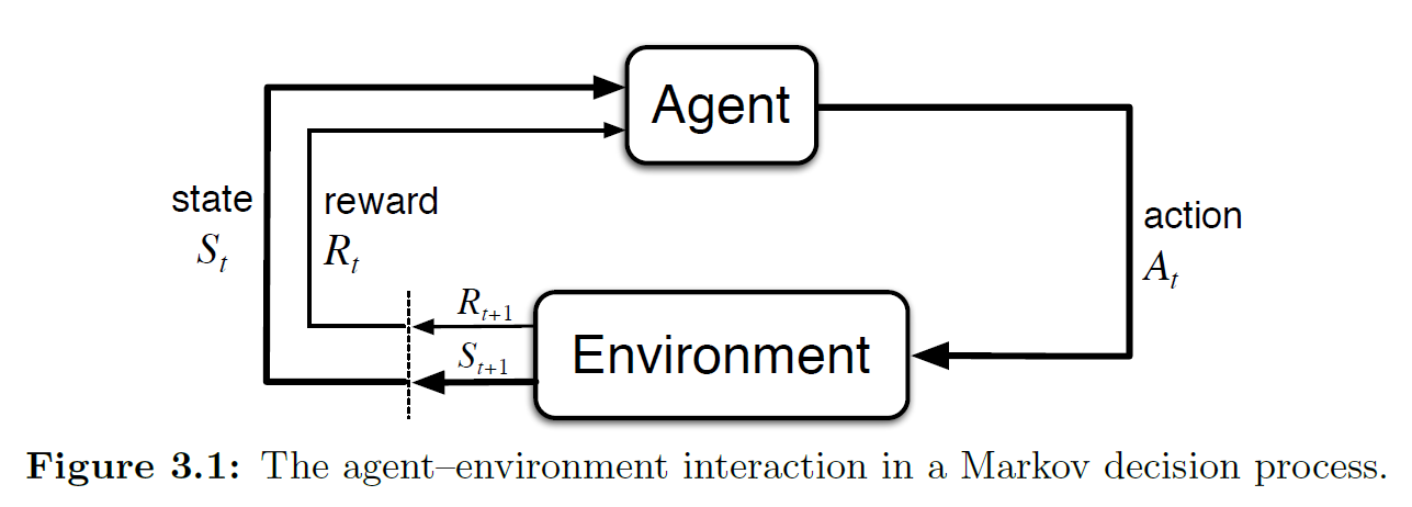
As shown in the figure above, the agent and environment interact continually: the agent selects actions, and the environment responds to those actions and presents new situations (i.e., states) to the agent. The environment also gives rise to rewards — special numerical values that the agent seeks to maximize over time through its choice of actions.
Let us restate this process: at each time step \(t\), the agent receives some representation of the environment's state \(S_t\). Based on this state, the agent selects an action \(A_t\). Then, after time step \(t\), the agent has completed this action, the time step advances to \(t+1\), and the environment returns a reward \(R_{t+_1}\) based on the action at \(t\) and writes it into the new state \(S_{t+1}\). The trajectory is as follows:
In a finite MDP, the sets of states \(\mathcal{S}\), actions \(\mathcal{A}\), and rewards \(\mathcal{R}\) are all finite. In this case, the random variables \(R_t\) and \(S_t\) have discrete distributions that depend only on the preceding state and action. This gives rise to the four-argument \(p\) function:
This function is the dynamics of the MDP, commonly referred to as the \(p\) function or the four-argument form of the \(p\) function, and is the form used most frequently throughout this book.
Since the four-argument function \(p(s',r|s,a)\) shown above is a joint probability distribution, for each state–action pair \((s,a)\), the joint probabilities over all possible next states \(s'\) and rewards \(r\) must sum to one:
For those who need a refresher on probability theory: a joint probability distribution describes the probability that two or more random variables simultaneously take certain values. For example, if you flip a coin and roll a die at the same time, \(P(\text{heads}, \text{result}=3)\) is a joint probability. So for Equation 3.3 above, given state \(s\) and action \(a\) — that is, after the agent takes action \(a\) in state \(s\) — the probability of the environment returning a new state \(s'\) and a reward \(r\) jointly is what is being described. As for why it sums to one: just as when you flip a coin and roll a die, the combination of all possible coin outcomes and all six die results must cover all possibilities, i.e., the total probability is 100%.
At the same time, we can see that in a Markov decision process, the future state of the system depends only on the current state and action, and not on any earlier states or actions. This property is called the Markov property. This property is extremely important because it imposes a constraint on what constitutes a "state": the state must contain all information that could affect future outcomes. Throughout most of this book, particularly before the discussion of approximation methods, we will assume that states possess the Markov property.
We must take the Markov property seriously, because if it does not hold, then algorithms designed on the basis of Markov decision processes (such as Q-learning, Policy Gradient, DQN) will produce incorrect estimates of the current state, the learned policy will fail, and the consequences can be severe. Here are some examples to illustrate:
| # | State Description | Markov? | Explanation |
|---|---|---|---|
| 1 | Current board position (e.g., Go, chess) | Yes | The current position contains all information relevant to winning or losing; no history needed |
| 2 | Current coordinates in a maze | Yes | Coordinates are sufficient for position-based decisions |
| 3 | Current video frame (no history) | No | Missing velocity, direction, etc.; cannot determine dynamic behavior |
| 4 | Current frame + previous frame | Approx. yes | Frame differencing can estimate velocity, reasonably approximating Markov property |
| 5 | Current stock price | No | Price trends depend on past information; current price alone is insufficient to predict future movement |
| 6 | Last 10 days of stock prices | Approx. yes | Contains some historical context, can approximately serve as a Markov state |
| 7 | Character HP + position + enemy status in a game | Yes | Contains all decision-relevant current information |
| 8 | Only player HP (no position, no enemy info) | No | State information is incomplete; future is uncertain |
| 9 | Agent's previous observation and action (no current observation) | No | Without the current state, the next step cannot be accurately predicted |
| 10 | Current sensor readings + internal hidden state (e.g., LSTM hidden layer) | Approx. yes | Provides a degree of memory, suitable for partially observable environments, enhances Markov property |
Now that we understand the Markov property, if we want to focus on only one variable in the joint probability, we can examine its marginal probability.
If we marginalize out the reward \(r\) and retain only the state-transition probability over \(s'\), we obtain the state-transition probability function:
Next, we need to consider: after the agent selects action \(a\) in state \(s\), what is the expected reward? This value is not the actual reward, but the expected value of the reward from executing that action in the long run. We typically use the expected reward function for state–action pairs, \(r : \mathcal{S} \times \mathcal{A} \rightarrow \mathbb{R}\):
This formula is very important and is a core component of policy evaluation. Since we often care only about the expected reward rather than the full reward distribution, this formula provides a very convenient computation. For example, in value functions we frequently need this expected reward (this formula will be covered later; it is introduced here only to illustrate the importance of the expected reward function):
Similarly, we can compute the expected reward for state–action–next-state triples as a three-argument function \(r : \mathcal{S} \times \mathcal{A} \times \mathcal{S} \rightarrow \mathbb{R}\):
The above constitutes the main formulas of the MDP framework. Among them, the four-argument \(p\) function from Equation 3.2 appears most frequently in this book, while the other formulas are also used throughout.
The strength of the MDP framework lies in its flexibility. For example: time steps need not correspond to real-time changes — they can be any successive stages in a decision process; actions can be low-level voltage controls or high-level decisions like whether to attend graduate school; states can be low-level sensor readings, high-level symbolic descriptions of objects in a room, or even entirely subjective or mental content. Some actions may be purely mental, or may control what the agent chooses to think about.
In general, actions can be any decisions we want to learn how to make, and states can be any information we know that might be useful in making those decisions. It is especially worth noting that the boundary between agent and environment is usually not the physical boundary of a robot or animal body, but rather a boundary that lies much closer to the agent itself. For instance, a robot's motors, mechanical linkages, and sensors should generally be considered part of the environment. Likewise, a person's skeleton, muscles, and sensory organs should be considered part of the environment. Rewards are similar — in the MDP framework, they are considered part of the environment, even though intuitively they might not seem to be.
We generally follow this principle: anything that cannot be changed arbitrarily by the agent is considered to be outside of it and thus part of its environment.
We do not assume that everything in the environment is unknown to the agent. The agent may know the rewards and the computations associated with them, but we must treat the reward computation as external to the agent, because rewards define the task the agent faces and must lie beyond the agent's ability to alter at will.
This may seem convoluted, so here is an example: suppose the agent must solve a Rubik's cube. How the cube works is obviously transparent, yet it remains a difficult reinforcement learning task. Therefore, the agent–environment boundary represents not the limit of the agent's knowledge, but the limit of its absolute control.
The agent–environment boundary can be set on a case-by-case basis. In complex problems, multiple agents may operate simultaneously, each maintaining its own boundary. For example, one agent might make high-level decisions, while the states corresponding to those decisions are perceived and provided by another, lower-level agent. In practice, the agent–environment boundary is determined by our choice of states, actions, and rewards, thereby defining a specific decision-making task.
The MDP framework is a highly abstract representation of goal-directed learning from interaction. It proposes that regardless of the specific details of sensing, memory, and control mechanisms, and regardless of what the goal is, any goal-directed learning behavior can be reduced to three signals passing back and forth between agent and environment:
- One signal represents the choices made by the agent — the action
- One signal represents the basis on which the agent makes choices — the state
- One signal defines the agent's goal — the reward
This framework may not be sufficient to represent all decision-learning problems, but it has been proven to be broadly useful and applicable. In reinforcement learning, the specific states and actions vary enormously across different tasks, and the way they are represented can greatly affect learning performance. As a result, these representational choices are sometimes more of an art than a science.
Below are some examples:
| Task/Goal | Actions | States | Rewards |
|---|---|---|---|
| Autonomous driving (safe arrival) | Steering, acceleration, braking | Current position, speed, obstacles ahead, traffic light status | Obstacle avoidance, safe driving, reaching destination |
| Playing Super Mario | Move left/right, jump, attack | Current screen information, character position, enemy positions | Score, defeating enemies, clearing levels |
| Automated stock trading | Buy, sell, hold | Historical price trends, technical indicators, account balance | Investment returns (profit or loss) |
| Chatbot sustaining conversation | Reply with a sentence | Context, current input, emotional state | User satisfaction, maintaining conversation |
| Robotic arm grasping objects | Rotate joints, close gripper | Camera feed, target position, gripper position | Successfully grasping object |
| Cleaning robot covering a room | Move forward, turn, activate vacuum | Current map position, remaining battery, surrounding obstacles | Score for each newly covered area |
| Recommendation system improving CTR | Recommend a video/product | User profile, behavioral history, current time | Whether user clicks or purchases |
| Drone autonomous navigation | Ascend, descend, move forward, turn | Current altitude, obstacle positions, target coordinates | Proximity to target, obstacle avoidance |
| Personalized education platform | Push exercises, provide hints, adjust difficulty | Student answer records, current knowledge topic, time invested | Student grade improvement, sustained learning duration |
| Medical diagnosis optimization | Recommend tests, suggest treatments | Patient history, symptoms, lab results | Improved treatment outcomes, reduced misdiagnosis |
Throughout this book, we provide suggestions and examples for how to effectively represent states and actions, but our primary focus is on: once the representations of states and actions have been determined, how to learn the correct behavioral policy.
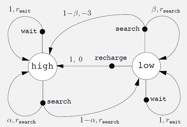
The book also provides three fairly detailed examples: Example 3.1 Bioreactor, Example 3.2 Pick-and-Place Robot, and Example 3.3 Recycling Robot. Example 3.3 is quite lengthy and provides a detailed illustration of how to model a real-world problem as a finite MDP.
In Example 3.3, the author presents a structure called a transition graph. This structure is covered in discrete mathematics and graph theory; interested readers can look up directed graphs, state transition diagrams, and related topics in graph theory. Graph theory can help with modeling, but not having studied it will not significantly impede learning reinforcement learning — after all, there are so many CS subjects that mastering even one area deeply is already a significant achievement.
Exercises 3.1–3.4: see the Appendix section.
3.2 Goals and Rewards
In reinforcement learning, the agent's goal is formalized through rewards. The reward is a special signal passed from the environment to the agent. At each time step, the reward is a simple number, denoted \(R_t \in \mathbb{R}\). This concept is a defining feature of reinforcement learning.
Informally, the agent's goal is to maximize the total reward it receives. In other words, the agent seeks to maximize long-term cumulative reward rather than immediate reward. This is the reward hypothesis:
That all of what we mean by goals and purposes can be well thought of as the maximization of the expected value of the cumulative sum of a received scalar signal (called reward).
In practice, this approach is widely applicable and commonly used. The book gives some examples that have been or could be employed:
- To teach a robot to walk, researchers give it a reward at each time step proportional to its forward velocity.
- To teach a robot to escape from a maze, the reward is typically −1 for every time step elapsed; this encourages the robot to escape as quickly as possible.
- To teach a robot to find and collect empty cans for recycling, the reward can be 0 most of the time, with +1 given only when a can is collected.
- We can also design negative rewards for the robot, such as deducting points when it bumps into things or is scolded by a person.
- For an agent learning to play checkers or chess, a natural reward scheme is: +1 for a win, −1 for a loss, and 0 for a draw or any non-terminal state.
In all these examples, the agent always learns to maximize its reward. If we want the agent to do something for us, we must set up the rewards in such a way that the agent, in maximizing its reward, also achieves our goal.
Therefore, the key lies in how to set the rewards so that they accurately reflect our goals. It is important to note that the reward signal is not meant to convey prior knowledge to the agent about how to achieve our goal. For example, for a chess-playing agent, we should only reward it for actually winning, not for achieving subgoals (such as capturing pieces). If these subgoals were rewarded, the agent might find ways to achieve them while ignoring the real objective. For instance, it might find ways to capture pieces quickly but end up losing the game.
So, the reward signal is how you tell the agent what you want it to achieve, not how you want it to achieve it. When setting the reward signal, you should focus on what goal you want to accomplish, not on how to make the agent accomplish that goal.
3.3 Returns and Episodes
The agent's goal is to maximize the cumulative reward it receives over the long run. How is this goal formally defined? If we denote the rewards received after time step \(t\) as \(R_{t+1},R_{t+2},R_{t+3},...\), then the expected return \(G_t\) we seek to maximize is:
The final time step indicates that this expression has a definite endpoint, i.e., a finite process. The entire process is called an episode — for example, one game, one maze traversal. This formulation does not apply to continuing tasks that have no endpoint.
The terminal time step \(T\) is a random variable that typically varies from episode to episode. Sometimes we need to distinguish the set of states that includes the terminal state, denoted \(\mathcal{S}^+\), from the set that does not, denoted \(\mathcal{S}\).
When an episode terminates, the process enters a terminal state, after which it either resets to a standard starting state or randomly samples from a set of standard starting states. In other words, regardless of the outcome of the episode — even if the rewards differ — the next round starts from the same mechanism. Thus, these episodes formally terminate in the same terminal state, but with different terminal rewards.
We generally treat all episodes as ending in the same terminal state but with different outcome-dependent rewards. Tasks of this type are called episodic tasks.
In contrast, continuing tasks have no terminal state and are commonly used for continuous process control or long-lived robot applications.
For continuing tasks, considering numerical and optimization concerns, we introduce an important new concept: discounting. With discounting, the agent selects its actions to maximize the sum of discounted future rewards. Specifically, the agent selects action \(A_t\) to maximize the expected discounted return:
The parameter \(\gamma (gamma,\ 0 \le \gamma \le 1)\) is called the discount rate, and it determines the present value of future rewards. A reward received \(k\) time steps in the future is worth only \(\gamma^{k-1}\) times what it would be worth if received immediately. If \(\gamma < 1\), then as long as the reward sequence \(\{ R_k \}\) is bounded, the infinite series in the discounted return formula converges to a finite value.
This formula can also be applied to episodic tasks with finite time horizons by simply setting the terminal time step:
There is also a commonly used variant (mentioned in Exercise 3.6): if the task is something like pole-balancing where there is no reward until termination, at which point a single reward of \(-X\) is given, the formula can be substituted and simplified to:
This expression shows that the farther away from failure (\(T\)), the smaller the absolute value of the return; the reward occurs only at the moment of failure.
If \(\gamma=0\), then the agent cares only about immediate rewards, and its behavior is myopic. However, if each of the agent's actions affects only the immediate reward and not future rewards, then a myopic policy can still maximize the return.
In practice, though, maximizing only the immediate reward will limit the acquisition of future rewards, thereby reducing the total return.
As \(\gamma\) approaches 1, the optimization objective places increasingly greater weight on future rewards, and the agent's behavior becomes more farsighted.
In reinforcement learning theory, there is an important recursive relationship between returns at different time steps:
This definition applies to all time steps \(t<T\). If the interaction terminates at \(t+1\) — meaning there are no further rewards from \(t+1\) onward — we can still use the same recursive formula to compute the return \(G_t\), as long as we define \(G_T=0\) (where \(T\) is the terminal time step).
For example, suppose the task terminates at time step \(t = 100\). Then we can define \(G_{100} = 0\) and use the recursive formula to compute \(G_{99} = R_{100} + 0\). This trick simplifies both computation and programming and is very practical.
When the reward is nonzero and constant and \(\gamma<1\), the return is still finite. For example, when the reward is constantly +1, the return is:
Exercises 3.5–3.10 for this section: see the Appendix.
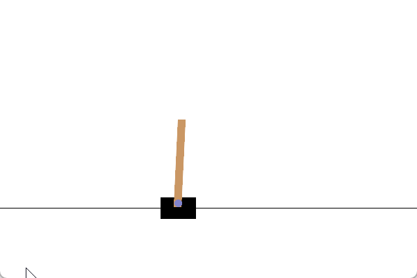
Note: In the exercises for this chapter, a classic pole-balancing problem is mentioned. The book does not require programming for this example, but given how classic this task is, an additional experimental section has been added to demonstrate how the material from this chapter can be applied in a practical setting. This section is placed in the Appendix under Programming 3.1: Pole-Balancing. Interested readers are welcome to take a look.
3.4 Unified Notation
In the previous section we discussed episodic tasks and continuing tasks. In this section we unify the notation for both types of tasks (Unified Notation). In other words, we unify Equations 3.7 and 3.8.
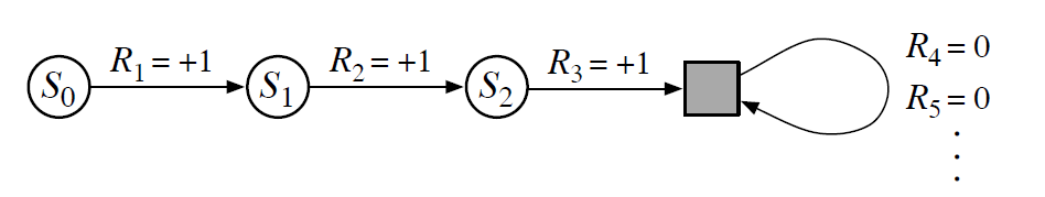
In the figure above (state transition diagram), the filled square represents the special absorbing state at the end of an episodic task. As a result, whether we sum only the first 3 steps of returns or sum all returns, the total return is the same.
That is, we can use the definition from Equation 3.8 to give the general return formula:
The reason both cannot hold simultaneously is to ensure that \(G_t\) converges.
3.5 Policies and Value Functions
Nearly all reinforcement learning algorithms involve estimating value functions — functions of states (or state–action pairs) that estimate how "good" it is for the agent to be in a given state, or how "good" it is to perform a given action in a given state. Here, "how good" is defined in terms of future rewards that can be expected — more precisely, in terms of the expected return. Of course, the rewards an agent can expect in the future depend on the actions it will take. Accordingly, value functions are defined with respect to particular ways of acting, called policies.
Formally, a policy is a mapping from states to probabilities of selecting each possible action. If the agent is following policy \(\pi\) at time \(t\), then \(\pi(a \mid s)\) is the probability that \(A_t = a\) given \(S_t = s\). Like \(p\), \(\pi\) is an ordinary function; the "\(|\)" in the middle merely reminds us that it defines a probability distribution over \(a \in \mathcal{A}(s)\) for each \(s \in \mathcal{S}\). Reinforcement learning methods specify how the agent's policy is changed as a result of its experience.
The state-value function under policy \(\pi\) is the expected return starting from state \(s\) and thereafter always following \(\pi\), denoted \(v_\pi(s)\). For MDPs, we can formally define \(v_\pi\) as:
Here \(\mathbb{E}_\pi[\cdot]\) denotes the expected value of a random variable given that the agent follows policy \(\pi\), and \(t\) is any time step. Note that the value of the terminal state (if any) is always zero. We call \(v_\pi\) the state-value function for policy \(\pi\).
Similarly, we define the value of taking action \(a\) in state \(s\) under policy \(\pi\), denoted \(q_\pi(s, a)\), as the expected return starting from state \(s\), taking action \(a\), and thereafter following policy \(\pi\):
We call \(q_\pi\) the action-value function for policy \(\pi\).
The value functions \(v_\pi\) and \(q_\pi\) can be estimated from experience. For example, if an agent follows policy \(\pi\) and maintains an average of the actual returns obtained after each visit to a state, this average will converge to \(v_\pi(s)\) as the number of visits to that state approaches infinity.
If we also maintain separate averages for each action taken in each state, those averages will likewise converge to the corresponding action values \(q_\pi(s, a)\). We call estimation methods based on averaging random sample returns Monte Carlo methods; these will be discussed in detail in Chapter 5.
Of course, if the number of states is very large, maintaining a separate average for each state becomes impractical. In such cases, the agent can maintain \(v_\pi\) and \(q_\pi\) as parameterized functions (with fewer parameters than states) and adjust the parameters to better match observed returns. Although the accuracy of such methods depends heavily on the nature of the function approximator used, they can also produce accurate estimates. Such possibilities are explored further in Part II of this book.
A fundamental property of value functions used in reinforcement learning and dynamic programming is that they satisfy recursive relationships similar to those established for the return in Equation 3.9. For any policy \(\pi\) and any state \(s\), the following consistency condition holds between the value of that state and the values of its successor states:
Using Equation 3.9, this can be further expanded as:
Since:
We finally obtain:
In the above expression, actions \(a\) come from the set \(\mathcal{A}(s)\), successor states \(s'\) come from \(\mathcal{S}\) (or possibly \(\mathcal{S}^+\) for episodic problems), and rewards \(r\) come from the set \(\mathcal{R}\).
Note that in the final formula, we merged the two sums over \(s'\) and \(r\) into a single sum over all \((s', r)\) pairs, in order to simplify the expression. This merged expression can in fact be understood as an expectation: we sum over all possible triples \((a, s', r)\), compute the probability \(\pi(a \mid s) p(s', r \mid s, a)\), multiply the bracketed expression by that probability, and sum over all possibilities to obtain the expectation.
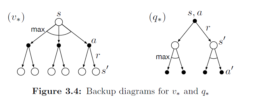
Equation (3.14) is the Bellman equation for \(v_\pi\). It expresses the relationship between the value of a state and the values of its successor states. It can be understood as: starting from a state, looking ahead to all possible successor states (as shown in the figure below).
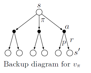
In the figure, each open circle represents a state, and each filled circle represents a state–action pair. Starting from the root state \(s\), the agent can choose among multiple actions according to policy \(\pi\) (three are shown in the figure). For each action, the environment may transition to some successor state \(s'\) (two are shown in the figure) and produce a reward \(r\); the probabilities of these transitions are described by the function \(p\).
The Bellman equation (3.14) takes a weighted sum over all possibilities, where the weights are the probabilities of occurrence. It states that: the value of a state equals the weighted sum of the rewards and discounted future values over all possible actions and successor states:
The value function \(v_\pi\) is the unique solution to its Bellman equation. In subsequent chapters, we will show how this Bellman equation serves as the foundation for many methods of computing, approximating, and learning \(v_\pi\).
We call these diagrams backup diagrams, because they visually illustrate the structure of update (or backup) operations that are central to reinforcement learning methods. These operations propagate value information backward to a state or state–action pair from its successor states (or state–action pairs).
We use backup diagrams throughout the book to provide graphical summaries of the various algorithms. (Note that unlike transition graphs, state nodes in backup diagrams do not necessarily represent distinct states; for instance, a state may be its own successor.)
For the Bellman equation, we can view it as different perspectives on the same MDP:
The Bellman equation for the state-value function, written out explicitly, can be expressed as:
The Bellman equation for the action-value function, written out explicitly, can be expressed as:
Depending on the specific application, the Bellman equation can be written flexibly when programming. Simply put, the Bellman equation combines the expected immediate reward with the expected future reward to yield an exact numerical solution.
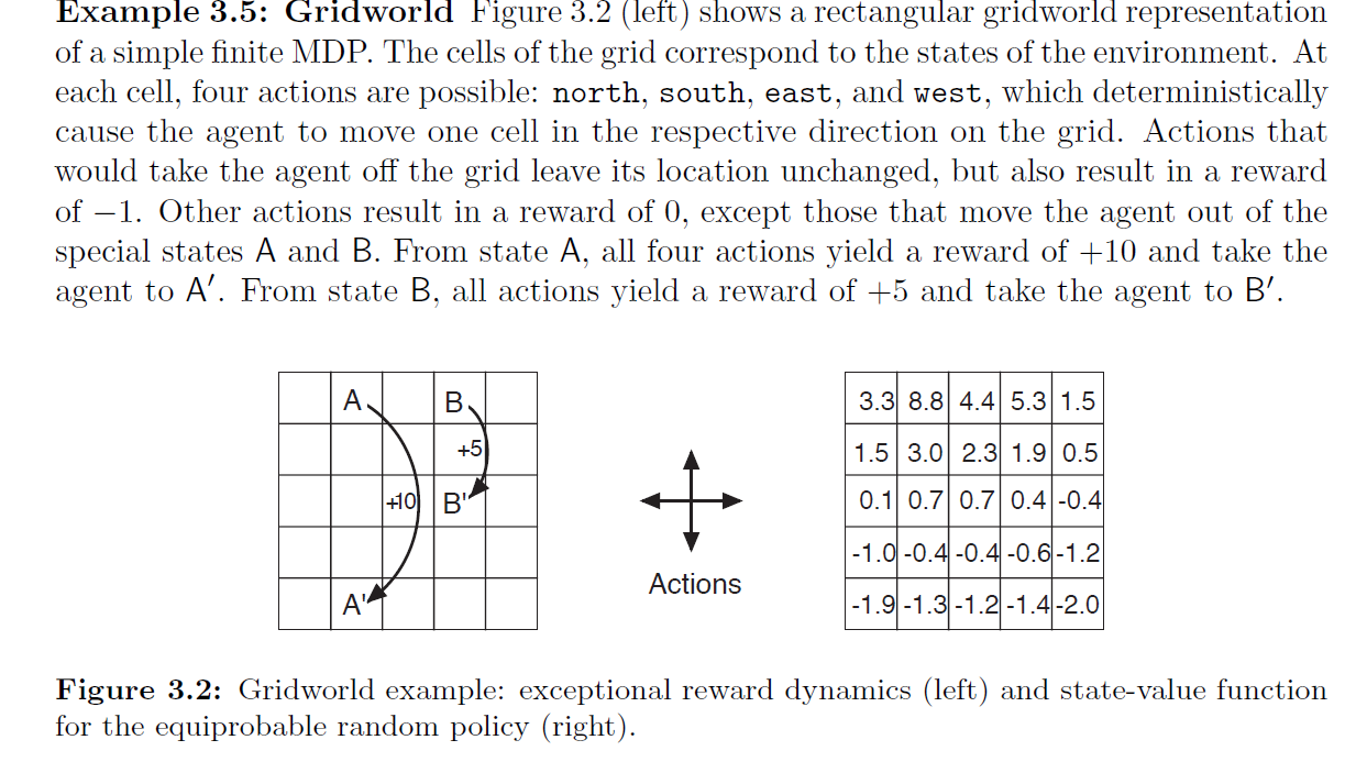
Example 3.5 Gridworld solution and programming: see Programming 3.2.
Example 3.6 on the golf putting problem is omitted. See p. 62 of the book for details.
Exercises 3.11–3.19 for this section: see the Appendix.
3.6 Bellman Optimality Equations
Solving a reinforcement learning task roughly means finding a policy that achieves a large amount of reward over the long run. For finite MDPs, we can precisely define an optimal policy as follows.
Value functions define a partial ordering over policies. A policy \(\pi\) is said to be better than or equal to another policy \(\pi'\) if its expected return is greater than or equal to that of \(\pi'\) for all states. In other words, \(\pi \geq \pi'\) if and only if \(v_\pi(s) \geq v_{\pi'}(s)\) for all \(s \in \mathcal{S}\).
There is always at least one policy that is better than or equal to all other policies. Such a policy is called an optimal policy. Although there may be more than one optimal policy, we denote all of them by \(\pi_*\). These optimal policies share the same state-value function, called the optimal state-value function, denoted \(v_*\), and defined as:
Optimal policies also share the same optimal action-value function, denoted \(q_*\), and defined as:
For a state–action pair \((s, a)\), this function gives the expected return for taking action \(a\) in state \(s\) and thereafter following an optimal policy. We can therefore express \(q_*\) in terms of \(v_*\) as:
The Bellman optimality equation for \(q_*\) is as follows:
The key thing to remember is that for finite MDPs, the Bellman optimality equation for \(v_*\) has a unique solution.
The Bellman optimality equation is a system of equations — one equation for each state. If the dynamics function \(p\) of the environment is known, then in principle we can use any of several nonlinear equation-solving methods to solve this system of equations for \(v_*\).
Once we have the optimal value function, a greedy policy with respect to it is an optimal policy. Because the system of equations we derived already accounts for long-term consequences, a greedy policy also means optimal in the long-term sense.
As for the action-value function, if we can obtain \(q_*\), then for any state \(s\) we simply need to find the action that maximizes \(q_*(s,a)\). In other words, given the optimal action-value function, the agent can directly make optimal action choices.
However, although the Bellman optimality equation is theoretically solvable, it is extremely difficult to apply in practice because it requires evaluating expected rewards over all possible paths — essentially an exhaustive search. Moreover, three major assumptions are required:
- The environment dynamics are known, i.e., \(p(s', r \mid s, a)\) is exact
- Sufficient computational resources are available to solve the nonlinear system of equations
- The state possesses the Markov property
As an example, chess has on the order of \(10^{43}\sim10^{50}\) states. Even with the most powerful supercomputer in 2025, solving for \(v_*\) would take an astronomical amount of time. Therefore, when solving practical problems, one must inevitably rely on approximate value functions and policies rather than solving the Bellman optimality equation directly.
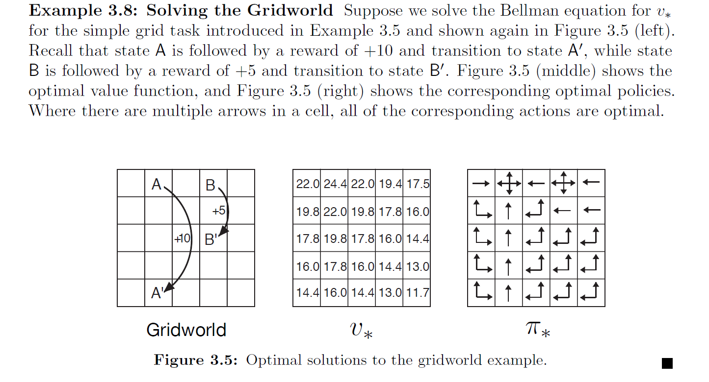
Examples 3.8, 3.10 from the book are omitted; Example 3.9: see Programming 3.2.
Exercises 3.20–3.29: see the Appendix.
3.7 Optimality and Approximation
Although in theory one can obtain the optimal policy by solving the Bellman optimality equation, for nearly all real-world problems this is infeasible. Therefore, optimality is a highly idealized condition, and for virtually all practical problems the agent can only achieve an approximation.
Consequently, the very nature of the reinforcement learning problem formulation dictates that function approximation is a central tool in reinforcement learning.
Reinforcement learning is capable of online policy updates, prioritizing optimization of states that are frequently encountered in practice. This is a major advantage of reinforcement learning over other methods when approximately solving MDPs. Specifically, the agent can immediately use newly obtained experience at each time step to update its policy or value function, rather than waiting until all data have been collected.
In the 1990s, TD-Gammon, based on temporal-difference learning (to be studied in Chapter 6), achieved world-class performance, defeating most human backgammon champions.
3.8 Summary
Let us summarize the elements of the reinforcement learning problem introduced in this chapter. The core of reinforcement learning is: learning how to act through interaction with the environment in order to achieve a goal. The agent in reinforcement learning interacts with its environment in discrete time steps. The definition of the environment interface determines a specific task:
- Actions are the choices made by the agent;
- States are the basis on which the agent makes its choices;
- Rewards are the basis for evaluating the outcomes of those choices.
Everything inside the agent is known and controllable, while the environment may be uncontrollable and may not be fully known. A policy is a stochastic rule by which the agent selects actions based on states. The agent's goal is to maximize the cumulative reward it receives.
When the reinforcement learning setup includes well-defined transition probabilities, it constitutes a Markov Decision Process (MDP). If it is a finite MDP, then the sets of states, actions, and rewards are all finite (this is the formulation used throughout this book). Most current reinforcement learning theory is based on finite MDPs, but many of the ideas apply equally in more general settings.
The return is a function of future rewards that the agent seeks to maximize (typically in expectation). It has several different definitions depending on the nature of the task and whether delayed rewards are discounted.
- The undiscounted form is suitable for episodic tasks, where the agent–environment interaction naturally breaks into separate episodes.
- The discounted form is suitable for continuing tasks, where the interaction has no natural endpoint and continues indefinitely (see Sections 10.3–10.4).
We have attempted to unify the notation for both types of tasks so that the same set of equations can apply to both episodic and continuing tasks.
The value functions of a policy (\(v_\pi\) and \(q_\pi\)) assign to each state or state–action pair an expected return — the expected return obtainable from that state or state–action pair given that the agent follows the policy.
The optimal value functions (\(v_*\) and \(q_*\)) assign to each state or state–action pair the maximum expected return achievable over all possible policies.
A policy whose value function equals the optimal value function is called an optimal policy. Although the optimal value function for state–action pairs is unique for a given MDP, there may be more than one optimal policy. Any policy that is greedy with respect to the optimal value function can be an optimal policy.
The Bellman optimality equations are a set of special constraints that the optimal value functions must satisfy. In principle, solving these equations yields the optimal value function, from which a corresponding optimal policy can be derived.
A reinforcement learning problem can be modeled from several different perspectives, depending on assumptions about the agent's initial knowledge.
- In the complete knowledge setting, the agent has a complete, accurate model of the environment dynamics. If the environment is an MDP, this model includes the complete four-argument state-transition function \(p\) (see Section 3.2).
- In incomplete knowledge problems, a complete and accurate model of the environment is not available.
Even when the agent has a complete and accurate model of the environment, it often cannot fully exploit it due to limitations in memory and computational power, especially when the computation available per time step is limited.
In practice, large amounts of memory may be needed to approximate value functions, policies, and models. In most problems of practical interest, the number of states far exceeds the available table capacity, so approximation is unavoidable.
A clear concept of optimality is the organizing core of the learning methods described in this book; it provides a way to understand the theoretical properties of various learning algorithms. But optimality is an ideal, and in practice, reinforcement learning agents can only achieve varying degrees of approximation.
Reinforcement learning is particularly concerned with situations in which the optimal solution cannot be obtained directly but can be progressively approximated.
Appendix: Exercises
Exercise 3.1 Designing Tasks
Q: Design three example tasks that fit the MDP framework, and for each, clearly identify the states, actions, and rewards. Make the three examples as different from each other as possible. Try to push the boundaries of the framework and expand its range of application.
A:
(1) Using reinforcement learning to teach a robot to navigate a maze
- Goal: Escape the maze
- States: The robot's surrounding environment, e.g., whether there are walls nearby
- Actions: Move forward, move backward, turn left, turn right
- Rewards: −1 for every second elapsed
(2) Using reinforcement learning for stock trading
- Goal: Achieve higher returns
- States: Overall stock market conditions
- Actions: Buy stocks, sell stocks
- Rewards: Higher monthly average returns yield higher rewards
(3) Teaching a robotic arm to grasp objects
- Goal: Have the robotic arm grasp an object and place it at a designated (fixed) location
- States: Arm posture, object position, gripper posture
- Actions: Arm movement, gripper grasping actions
- Rewards: Rewards for successful grasping and successful placement at the designated location
The author's examples above are fairly standard. ChatGPT generated some more creative designs for reference:
(1) AI Poetry Style Controller
- Goal: Generate poems with high emotional resonance and aesthetic quality
- States: Current poem's style vector (emotional tone, rhyme structure, current stanza, semantic embedding of the previous line)
- Actions: Adjust style parameters, switch themes, introduce symbolic techniques
- Rewards: +10 for emotional authenticity; +5 for natural rhyming; +20 for being bookmarked; −10 for jarring style shifts
(2) DNA Sequence Design Optimizer
- Goal: Design stable, well-expressed DNA sequence fragments for protein production
- States: Current sequence fragment's nucleotide composition, predicted biological function score, structural stability score
- Actions: Insert, delete, or replace a base pair
- Rewards: +50 for reaching target protein expression level; +20 for structural stability; −30 for toxicity or non-expression
(3) Improvisational Theater Actor Strategy Learning
- Goal: As an AI actor participating in improv, improve audience reactions and plot progression
- States: Current plot node, other characters' actions, audience emotion indicators
- Actions: Improvise character traits, introduce new plot conflicts, mimic other actors' styles
- Rewards: +15 for audience laughter/applause; +10 for advancing the plot; −10 for disrupting rhythm or creating dead air
(4) Consciousness Regulation Agent in a Meditation Guidance System
- Goal: Dynamically guide users into deeper meditation states through voice or prompts, achieving emotional stability and brainwave relaxation
- States: User's physiological state and environmental state, e.g., brainwaves, guidance intensity, ambient sound level
- Actions: Adjust speaking pace, insert natural sounds, add silent pauses, etc.
- Rewards: +20 for brainwaves entering deep meditation; −10 for user distraction or irritability
Author's aside: I did not expect ChatGPT's answers to be more imaginative and creative than mine. These AI-generated examples suddenly made me realize that if the entire human biological body could be migrated into a virtual world, reinforcement learning would experience explosive growth because large-scale experiments could be conducted with virtual human bodies. But this thought also feels somewhat dark — for example, in the theater strategy scenario, if a human-like entity were created, would it possess consciousness? And if we ran 5 million simulations, wouldn't that mean causing that entity to "die" 5 million times? This is an angle I had never considered before, and ChatGPT's examples suddenly made me realize that AI's moral and ethical framework will ultimately be fundamentally different from that of humans. Sutton's Bitter Lesson demonstrated the side effects of human experience in AI development; conversely, if AI development becomes independent of human consciousness and relies solely on computing power, algorithms, and the like, then if we truly create AGI, its moral and ethical framework will certainly not be equivalent to humanity's.
This question opens up further topics: Where are the ethical boundaries of simulating humans? Can subjective human experience be encoded? Should moral input be part of the reward? Is AGI's value system really learned from human experience?
What I appreciate most about Sutton is that he has always been thinking about philosophical questions regarding human intelligence and artificial intelligence. Hinton is the same — he is now traveling everywhere to raise awareness about the potential dangers of artificial intelligence. They are the founding figures of AI and are fully deserving of the title. I hope more practitioners will pay attention to ethical issues. We all know that AGI will inevitably be created; before that happens, we should give greater attention to its safety and ethics. Moreover, this technology must not be controlled by a single organizational entity — no wonder Hinton expressed his hope that "China and the US can achieve mutual balance" regarding the vigorous development of AI.
Exercise 3.2 Scope of the MDP
Q: Is the MDP framework adequate to usefully represent all goal-directed learning tasks? Can you think of any clear exceptions?
A:
First, the MDP framework is only applicable to tasks satisfying the Markov property: future states depend only on the current state, time steps are discrete, the environment is fully observable, and the transition and reward rules are fixed.
Examples where the MDP framework is not applicable:
- Navigating in fog, where the environment state cannot be fully observed
- A reward is given only for executing a specific sequence of actions
- Asynchronous events, such as another vehicle suddenly changing lanes in autonomous driving
- Multi-agent environments where, from each agent's perspective, the environment is non-stationary (e.g., StarCraft)
- Hierarchical goals, such as cooking braised pork which involves multiple sub-tasks like cutting meat and cooking rice
Exercise 3.3 The Agent–Environment Boundary
Q: Consider the most common driving problem. You can define "actions" as acceleration, steering, braking, etc. — in which case the actions occur where your body interacts with the machine. You could also consider the torques applied at the tires' contact with the road as the actions. Alternatively, actions could be your body's muscle control commands. We could even say the action is choosing where to drive. As you can see, distinguishing actions from the environment is highly subjective. What is the right level, the right place to draw the line between agent and environment? On what basis is one location of the line to be preferred over another? Is there any fundamental reason for preferring one location over another, or is it a free choice?
A: This is an open-ended thinking question, and one that Sutton often contemplates. There is no single correct answer; different action definitions depend on the task objective we wish to solve. This is also an important reason why reinforcement learning differs from today's popular LLMs. In reinforcement learning, the task objective itself constrains this boundary, and the complexity and feasibility of modeling further influence how actions are defined. Additionally, whether data can be obtained also affects the action definitions.
Exercise 3.4 Trace Table
This exercise asks you to produce a table similar to the one in Example 3.3, for the four-argument state-transition function.
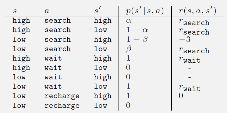
The original table is shown in the figure. This exercise is worth trying on your own when you first solve a real problem, so it will not be elaborated here.
Exercise 3.5
Q: The formula from Section 3.1 applies to continuing tasks:
How should it be modified for episodic tasks?
A: This equation states that after executing action \(a\) in state \(s\), the probabilities of all possible next-state-and-reward combinations must sum to one. In episodic tasks, there is no "next state" after the terminal state, so we introduce new notation:
The equation is then modified to:
That is, we must allow \(s'\) to be the terminal state, using \(\mathcal{S}^+\) to denote all ordinary states plus the terminal state.
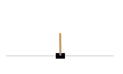
Exercise 3.6 Pole-Balancing

Pole-balancing is a very classic reinforcement learning task. The goal is to apply forces to a cart moving on a track so that a pole attached to the cart remains upright and does not fall over.
If the pole deviates from vertical beyond a given angle, or if the cart runs off the track, it is considered a failure. After failure, the state is reset.
This task can be viewed as an episodic task, where the natural episodes are successive attempts at balancing the pole. At each non-failure time step, the reward is +1, so the return at each time point is the number of time steps before failure. In this case, if the pole is balanced indefinitely (never fails), the return tends toward infinity.
An alternative is to treat pole-balancing as a continuing task using discounting. In this case, each failure incurs a reward of −1, with a reward of 0 at all other time steps. The return at each time point is then related to \(-\gamma^{K-1}\), where \(K\) is the number of time steps until failure occurs (which may also include subsequent failure time points). Under both formulations, the return-maximizing policy is to keep the pole balanced for as long as possible.
Note that there are generally two conventions for recording task failure: one uses \(T\) to denote the time step at which the task fails; the other records \(K\) as the episode length (counting from time step 0), with \(K-1\) being the last valid time step — the moment failure occurs.
Exercise 3.6 asks: Suppose you treat the pole-balancing task as an episodic task but also use discounting, and all time-step rewards are 0, with only a reward of −1 at failure. What should the return be at each time point? How does this return differ from the "discounted continuing task" formulation described above?
A:
(1) If all time-step rewards are 0 and only the failure reward is −1, then with \(t\) as the current time step, \(T\) as the terminal time step, and discount factor \(\gamma \in (0,1]\), the return in the current episode is:
This return accurately reflects how long balance was maintained in a single attempt, and the later the failure, the smaller the penalty. As the agent improves, the return for each episode also improves (less penalty).
(2) Meanwhile, if the environment does not reset, the agent runs forever and failure may occur many times. The return is the discounted sum of all future failure penalties:
By the standard discounted return definition for continuing tasks:
If a failure occurs at time \(K\), i.e., \(R_K = -1\), then to determine its contribution to \(G_t\), let:
So that failure's contribution to \(G_t\) is:
That is:
Exercise 3.7
Q:
Suppose you are designing a robot to navigate a maze. You decide on the following reward scheme: +1 for successfully escaping the maze, and 0 at all other times. The task naturally breaks into episodes — successive maze-traversal attempts — so you model it as an episodic task, aiming to maximize the expected total reward (Equation 3.7).
After running the learning agent for a while, you find that it shows no improvement at escaping the maze.
Think about: what is the problem? Have you truly communicated your objective clearly to the agent?
A:
Clearly, as long as the agent eventually escapes the maze, it receives a reward of +1. This design does not reward escaping quickly, so naturally there is no incentive for improvement. The correct approach should penalize the agent for taking longer, for example, giving a reward of −1 for each second spent in the maze. This way, the agent is motivated to minimize the number of steps spent in the maze.
Another approach is to use a discount factor to reduce the value of delayed rewards.
Exercise 3.8
Suppose the discount factor \(\gamma = 0.5\) and you receive the following reward sequence:
The terminal time is \(T = 5\). Compute the following returns:
A:
By Equation 3.9:
To compute \(G_t\), we must first compute \(G_{t+1}\), so we work backward from the end.
Since \(T=5\), we have \(G_T=G_5=0\).
1. Compute \(G_4\):
2. Compute \(G_3\):
3. Compute \(G_2\):
4. Compute \(G_1\):
5. Compute \(G_0\):
Final results:
Exercise 3.9
Suppose \(\gamma = 0.9\) and the reward sequence is \(R_1 = 2\) followed by an infinite sequence of 7s. What are \(G_1\) and \(G_0\)?
Suppose the discount factor \(\gamma = 0.9\), and the reward sequence is
followed by infinitely many
Compute the returns
A:
Using Equations 3.10 and 3.9, we can compute directly:
-
Compute \(G_1\)
Starting from \(t=1\), all subsequent rewards are 7, so
$$ G_1 = \sum_{k=0}^{\infty} \gamma^k \cdot 7 = 7 \sum_{k=0}^{\infty} (0.9)^k = 7 \times \frac{1}{1 - 0.9} = 7 \times 10 = 70. $$ 2. Compute \(G_0\) Starting from \(t=0\), the first reward is \(R_1=2\), followed by infinitely many 7s, so
$$ G_0 = R_1 + \gamma\,G_1 = 2 + 0.9 \times 70 = 2 + 63 = 65. $$
Therefore the final answers are:
Exercise 3.10 – 3.13
Exercise 3.10
Prove Equation 3.10. This proof can be found in Appendix: Math, section Math 3.1.
Exercise 3.11
If the current state is \(S_t\), and actions are selected according to a stochastic policy \(\pi\), then what is the expectation of \(R_{t+1}\) in terms of \(\pi\) and the four-argument function \(p\) (3.2)?
Answer:
By the definition of the four-argument transition function:
Since actions are sampled according to policy \(\pi\), we take the expectation over all possible actions and outcomes:
Exercise 3.12
Give an equation for \(v_\pi\) in terms of \(q_\pi\) and \(\pi\).
Answer:
The state-value function is the weighted average of the action-value function, where the weights are the policy's selection probabilities for each action in that state:
Exercise 3.13
Give an equation for \(q_\pi\) in terms of \(v_\pi\) and the four-argument \(p\).
Answer:
The action-value function represents the expected return from taking action \(a\) in state \(s\), and can be expressed as:
Exercise 3.14 – 3.19
Exercise 3.14
For the Gridworld in Example 3.5 (i.e., Programming 3.2), numerically verify whether the Bellman equation holds for the center cell:
A:
Given:
- Policy \(\pi\) selects among the four actions (up, down, left, right) with equal probability: \(\pi(a \mid s) = \frac{1}{4}\)
- The environment is deterministic; each cell's actions have definite outcomes
- Discount factor \(\gamma=0.9\)
By the Bellman equation:
To compute the value of the center state \(s_c\):
From the figure, the values of the four neighbors of the center cell can be read off and substituted:
This matches the value shown for the center cell in the figure. For a more detailed explanation and code experiment, see Programming 3.2.
Exercise 3.15
In the Gridworld example, reaching the goal yields a positive reward, hitting the edge of the world yields a negative reward, and the reward is zero otherwise. Consider: are the signs of these rewards important, or only the intervals (differences) between them?
Using Equation (3.8), prove that if a constant \(c\) is added to all immediate rewards, the value function of every state increases by the same constant \(v_c\), so the relative values among states are unaffected under any policy.
Q: What is \(v_c\) expressed in terms of the constant \(c\) and the discount factor \(\gamma\)?
A: Clearly, we define the cumulative return as:
If a constant \(c\) is added to every step's reward, defining the new reward as:
then the corresponding new return is:
And:
So the additional term is:
Therefore, adding a constant to all state values does not affect the relative values between different states; it merely shifts the entire value function vertically, by an amount of \(c/({1-\gamma})\). Note: this conclusion applies only to continuing tasks; for episodic tasks, see the next exercise.
Exercise 3.16
Now consider adding a constant \(c\) to all immediate rewards in an episodic task (e.g., maze running).
- Does this affect the task itself?
- Or does it leave the task unchanged, as in a continuing task? Explain why, and give a concrete example.
A:
The discounted return for an episodic task (from \(t\) to terminal time \(T\)):
Adding a constant \(c\) to every step's immediate reward:
The effect on the state-value function:
After adding the constant:
We therefore obtain:
From the above, in a continuing task where \(T \to \infty\) and \(0 \leq \gamma < 1\), we have \(\gamma^{T - t} \to 0\), so \(\Delta(s) = 1\) for all states, giving:
which simply adds the same constant to all states and does not change the relative ordering.
In an episodic task, \(\gamma^{T - t}\) varies with the "steps to termination" \(T - t\), so \(\Delta(s)\) depends on state \(s\) (or the average remaining episode length under policy \(\pi\)). Different states therefore receive different offsets, which can change the relative magnitudes of state values and thus affect the optimal policy.
Exercises 3.17–3.19 are temporarily omitted; they concern the Bellman equation and can be found on pp. 61–62 of the book.
Exercise 3.20 – 3.29
Exercises for the Bellman optimality equation chapter. Omitted for now; to be completed later.
Appendix: Programming
Programming 3.1 Pole-Balancing
In this section, we describe how to use Gymnasium for reinforcement learning experiments.
Gymnasium is a project that maintains classic experimental environments commonly used in reinforcement learning, succeeding the now-deprecated Gym project.
In Chapter 2, we learned about the experimental implementation of the bandit problem. However, the bandit problem has no concept of state — each action immediately ends the trial, and the action value is estimated using sample-average updates:
Although we have not yet covered Monte Carlo Methods, we can easily extend the sample-average update above to include states:
The Gymnasium environment page can be found here.
For this experiment, the state space is:
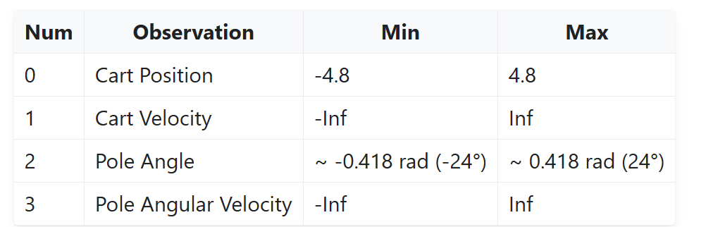
The action space is:
- 0: Push cart to the left
- 1: Push cart to the right
The environment provides two built-in reward settings:
- Sutton_Barto_Reward=True: as discussed, 0 before termination and −1 at termination
- Alternatively, +1 at every time step; the threshold in v1 is 500
Hyperparameters and training setup are as follows:
- Discount factor \(\gamma = 0.99\)
- Exploration rate \(\epsilon = 0.1\) (during training); set to \(\epsilon = 0\) during demonstration
- Learning rate: \(\displaystyle \alpha_t = \frac{1}{N(s,a)}\) (sample-average update)
- Training episodes: episodes = \(500\)
- Maximum steps per episode: environment default \(500\) steps
- Policy execution (sampling)
During training, an \(\epsilon\)-greedy policy is used:
During demonstration, a pure greedy policy is used: \(\epsilon = 0\).
- Data collection: each episode starts from
env.reset(), withenv.step(action)called in a loop until failure or maximum steps reached. -
Discounted return computation: for trajectory \((s_t, a_t, r_{t+1})_{t=0}^{T-1}\), compute
$$ G_t = \sum_{k=0}^{T-1-t} \gamma^k\,r_{t+1+k}. $$ - Q-table sample-average update:
\[ N(s_t,a_t) \leftarrow N(s_t,a_t) + 1, \]\[ Q(s_t,a_t) \leftarrow Q(s_t,a_t) + \frac{1}{N(s_t,a_t)}\bigl(G_t - Q(s_t,a_t)\bigr). \]
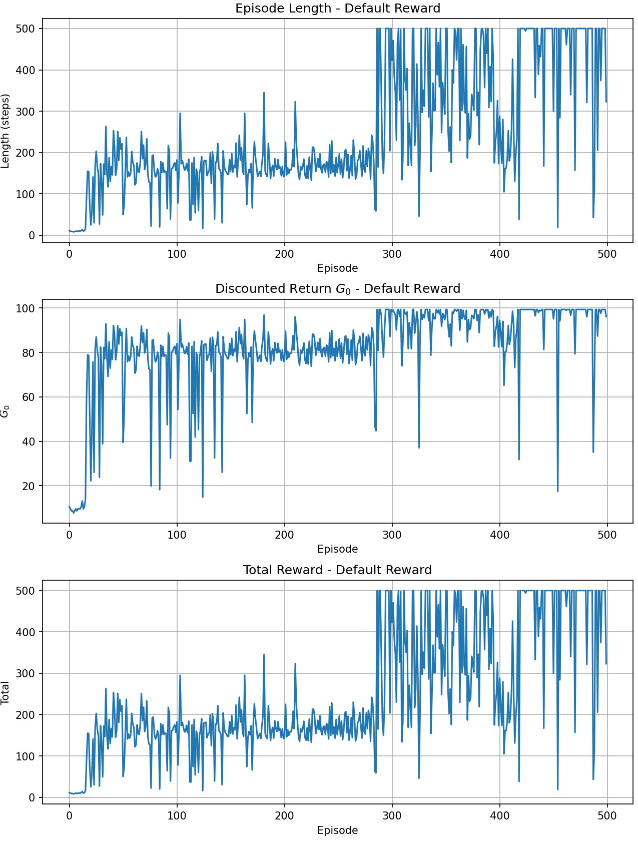
Results:
- Plot total return curves under both reward modes (500 episodes).
- Demonstrate the optimal (greedy) policy animation under Sutton–Barto mode and output example returns.
The post-training results are shown below:
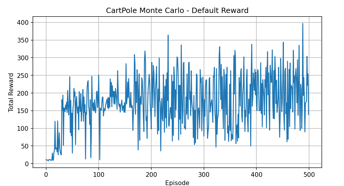
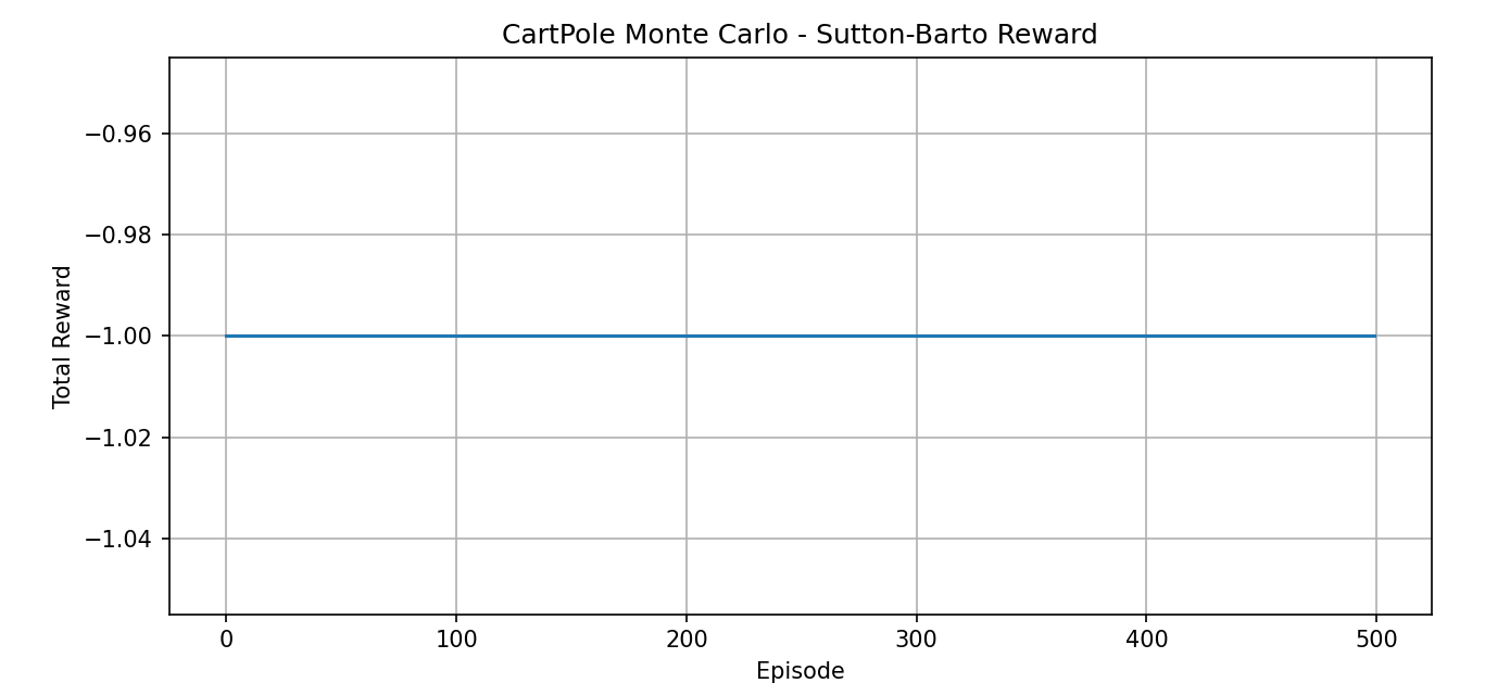
Here we observe that if we use the Chapter 2 bandit-style reward plot, the Sutton-Barto method produces a flat line because the final reward is always −1. In principle, the two methods produce the same result — they both use the same policy to maximize the pole's survival time \(T\) — but they differ in numerical scale, variance, and convergence speed:
- The reward method provides a continuously accumulating, relatively large positive signal for the return
- The Sutton-Barto method provides a decaying negative signal
Therefore, I modified the code to show results from multiple perspectives (since no random seed was used, each training run differs, which is why the Reward plot for the reward method differs slightly from the one above):
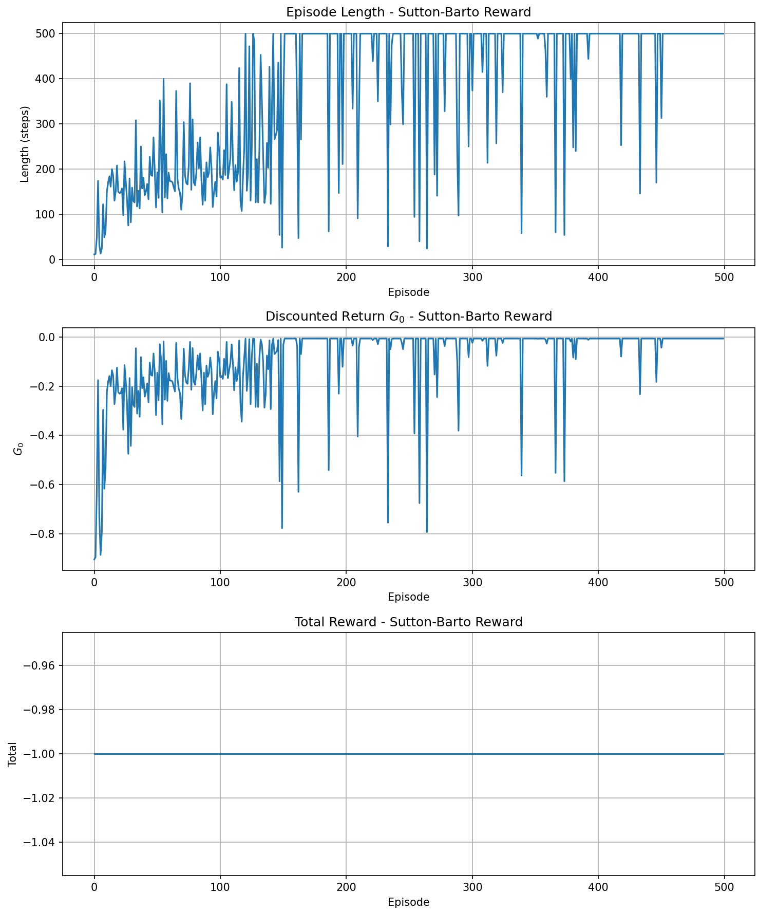
Finally, here is a demonstration of the trained result (Sutton-Barto method):
Code: see Appendix, Code section, Code 3.1.
Programming 3.2 Gridworld
This example corresponds to Example 3.5 from the book.
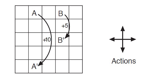
As shown in the figure, in this grid world, the only available actions are moving up, down, left, and right. If a move would take the agent off the grid, a reward of −1 is given and the agent stays in place. Special state A yields +10 and teleports to A'; special state B yields +5 and teleports to B'. All other actions yield a reward of 0.
Given this figure, we solve for the state-value distribution of each cell in the grid world.
Let us examine the MDP corresponding to this example:
- Finite state space: 25 cells correspond to 25 states
- Deterministic transitions: each action leads to a unique successor state
- Fixed reward function distribution
- (Standard setting used in the book) \(\gamma=0.9\)
Since the state transitions and reward function are fixed and we can solve exactly, the resulting state-value distribution is necessarily unique.
Let us first construct this Gridworld:
 0  1  2  3  4
 5  6  7  8  9
10 11 12 13 14
15 16 17 18 19
20 21 22 23 24
Next, define the state-transition function:
def step(s, a):
    if s == 1: return 21, 10   # A
    if s == 3: return 13, 5    # B
    i, j = s // 5, s % 5
    if a == 0: i2, j2 = i-1, j      # up
    if a == 1: i2, j2 = i+1, j      # down
    if a == 2: i2, j2 = i, j-1      # left
    if a == 3: i2, j2 = i, j+1      # right
    if i2 < 0 or i2 > 4 or j2 < 0 or j2 > 4:
        return s, -1  # hit wall
    return i2*5 + j2, 0  # move
Then adopt a uniform random policy:
The reason it is 1/4 is that four actions are available in every state, and we are using an equiprobable random policy, so the four action choices in each state are uniform.
Next, for each state \(s\), write out:
Which is:
With 25 states, this gives 25 linear equations.
The pseudocode is as follows (for the actual code, see Code 3.2 in the Code Appendix):
1. Initialization:
   - Grid size 5x5, total of 25 states
   - Discount factor gamma = 0.9
   - Four actions per state: up, down, left, right
   - Define special states A and B with their reward and teleportation rules

2. Define state-transition function step(s, a):
   - If current state is A or B, return the corresponding teleport state and special reward
   - Otherwise move one cell in the action direction; if hitting a wall, stay in place with -1 reward

3. Build the Bellman equation system (Av = b):
   - Initialize coefficient matrix A and constant vector b to zeros
   - For each state s:
       For each action a:
           - Get successor state s' and immediate reward r from step(s, a)
           - Add 0.25 * gamma to A[s, s'] (uniform policy)
           - Add 0.25 * r to b[s]
       - Subtract 1 from A[s, s] to move all terms to the left side

4. Solve the linear system Av = b to get v(s) for each state

5. Reshape the result into a 5x5 grid and output each cell's state value
Running the code gives the following result:
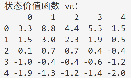
At this point, we have completed the "evaluation" of this problem — that is, given a policy, we have obtained its state-value function. (This step is generally called policy evaluation.)
Through the above solution, we found the expected value at each cell, representing the weighted average return over all directions when acting according to the current policy (equiprobable in all four directions).
To obtain a more detailed solution — namely, the values corresponding to each of the four directions at each cell — we need to compute the state-action value function.
In Section 3.5 of the book, after introducing the Bellman optimality equation, the specific solution for Gridworld is presented.
Appendix: Math
Math 3.1
Prove: the right-hand side of Equation 3.10, i.e., the following geometric series identity holds for \(0 \leq \gamma < 1\):
Proof:
Consider the infinite series:
This is a geometric series with common ratio \(\gamma\). We use the following geometric series summation formula (valid for \(|\gamma| < 1\)):
Substituting directly gives:
Alternative algebraic proof (constructive method):
Let:
Multiply both sides by \(\gamma\):
Subtracting the two equations:
QED.
math 3.2
Appendix: Code
Code 3.1 Cart-Pole Balancing
import gymnasium as gym
import numpy as np
import matplotlib.pyplot as plt

class CartPoleEnvironment:
    """
    CartPole environment wrapper with discretization and optional Sutton-Barto reward and rendering.
    """
    def __init__(self,
                 n_bins=(6, 6, 12, 12),
                 obs_bounds=((-4.8, 4.8), (-5, 5), (-0.418, 0.418), (-5, 5)),
                 sutton_barto_reward=False,
                 render_mode=None):
        self.env = gym.make("CartPole-v1", render_mode=render_mode)
        self.sutton_barto = sutton_barto_reward
        self.n_bins = n_bins
        self.bins = [np.linspace(low, high, bins - 1)
                     for (low, high), bins in zip(obs_bounds, n_bins)]

    def discretize(self, obs):
        return tuple(np.digitize(obs[i], self.bins[i]) for i in range(len(obs)))

    def reset(self, seed=None):
        obs, _ = self.env.reset(seed=seed)
        return self.discretize(obs)

    def step(self, action):
        obs, reward, terminated, truncated, _ = self.env.step(action)
        done = terminated or truncated
        if self.sutton_barto:
            reward = -1 if done else 0
        return self.discretize(obs), reward, done

class MonteCarloAgent:
    """
    On-Policy Monte Carlo Control agent with epsilon-greedy policy.
    """
    def __init__(self, n_bins, n_actions, epsilon=0.1, gamma=0.99):
        self.n_bins = n_bins
        self.n_actions = n_actions
        self.epsilon = epsilon
        self.gamma = gamma
        self.Q = np.zeros(n_bins + (n_actions,))
        self.N = np.zeros(n_bins + (n_actions,), dtype=int)

    def choose_action(self, state, greedy=False):
        if not greedy and np.random.rand() < self.epsilon:
            return np.random.randint(self.n_actions)
        return int(np.argmax(self.Q[state]))

    def update(self, episode):
        # Compute discounted returns for the episode
        G = 0
        returns = []
        for state, action, reward in reversed(episode):
            G = reward + self.gamma * G
            returns.insert(0, G)
        # Sample-average update of Q
        for (state, action, _), Gt in zip(episode, returns):
            self.N[state + (action,)] += 1
            alpha = 1.0 / self.N[state + (action,)]
            self.Q[state + (action,)] += alpha * (Gt - self.Q[state + (action,)])


def main():
    episodes = 500
    stats = {
        'Default': {'lengths': [], 'returns': [], 'totals': []},
        'Sutton-Barto': {'lengths': [], 'returns': [], 'totals': []}
    }

    # Training both modes
    for mode, sb in [('Default', False), ('Sutton-Barto', True)]:
        env = CartPoleEnvironment(sutton_barto_reward=sb)
        agent = MonteCarloAgent(env.n_bins, env.env.action_space.n,
                                epsilon=0.1, gamma=0.99)
        for ep in range(episodes):
            state = env.reset(seed=ep)
            episode = []
            steps = 0
            total_reward = 0
            done = False
            while not done:
                action = agent.choose_action(state)
                nxt, r, done = env.step(action)
                episode.append((state, action, r))
                state = nxt
                total_reward += r
                steps += 1
            # Record metrics
            stats[mode]['lengths'].append(steps)
            # Discounted return G0
            G0 = 0
            for (_, _, r) in reversed(episode):
                G0 = r + agent.gamma * G0
            stats[mode]['returns'].append(G0)
            stats[mode]['totals'].append(total_reward)
            agent.update(episode)

    # Plot Default Reward metrics
    fig, axes = plt.subplots(3, 1, figsize=(10, 12))
    axes[0].plot(stats['Default']['lengths'])
    axes[0].set_title('Episode Length - Default Reward')
    axes[0].set_xlabel('Episode')
    axes[0].set_ylabel('Length (steps)')
    axes[0].grid(True)

    axes[1].plot(stats['Default']['returns'])
    axes[1].set_title('Discounted Return $G_0$ - Default Reward')
    axes[1].set_xlabel('Episode')
    axes[1].set_ylabel('$G_0$')
    axes[1].grid(True)

    axes[2].plot(stats['Default']['totals'])
    axes[2].set_title('Total Reward - Default Reward')
    axes[2].set_xlabel('Episode')
    axes[2].set_ylabel('Total')
    axes[2].grid(True)

    plt.tight_layout()
    plt.show()

    # Plot Sutton-Barto Reward metrics
    fig, axes = plt.subplots(3, 1, figsize=(10, 12))
    axes[0].plot(stats['Sutton-Barto']['lengths'])
    axes[0].set_title('Episode Length - Sutton-Barto Reward')
    axes[0].set_xlabel('Episode')
    axes[0].set_ylabel('Length (steps)')
    axes[0].grid(True)

    axes[1].plot(stats['Sutton-Barto']['returns'])
    axes[1].set_title('Discounted Return $G_0$ - Sutton-Barto Reward')
    axes[1].set_xlabel('Episode')
    axes[1].set_ylabel('$G_0$')
    axes[1].grid(True)

    axes[2].plot(stats['Sutton-Barto']['totals'])
    axes[2].set_title('Total Reward - Sutton-Barto Reward')
    axes[2].set_xlabel('Episode')
    axes[2].set_ylabel('Total')
    axes[2].grid(True)

    plt.tight_layout()
    plt.show()

    # Demonstrate Sutton-Barto policy
    demo_env = CartPoleEnvironment(sutton_barto_reward=True, render_mode='human')
    state = demo_env.reset()
    done = False
    print("Demonstrating Sutton-Barto policy...")
    while not done:
        action = agent.choose_action(state, greedy=True)
        state, _, done = demo_env.step(action)
    demo_env.env.close()

if __name__ == '__main__':
    main()