Seq2Seq
The Sequence-to-Sequence model was independently proposed by Sutskever et al. (2014) and Cho et al. (2014). It was the first neural network architecture to successfully handle the variable-length input → variable-length output problem. It pioneered the Encoder-Decoder paradigm, which was later inherited and greatly advanced by the Transformer.
Why Do We Need Seq2Seq?
In the RNN and LSTM notes, we encountered several input-output structures:
- Many-to-One (sentiment analysis): takes a sequence as input, outputs a single label
- Many-to-Many synchronized (NER): input and output have the same length, with one-to-one correspondence
However, many tasks involve inputs and outputs of different lengths, and the output length cannot be known in advance:
| Task | Input | Output | Length Relationship |
|---|---|---|---|
| Machine Translation | "我喜欢猫" (3 words) | "I like cats" (3 words) | May or may not be the same |
| Text Summarization | A 1000-word article | A 50-word summary | Output much shorter than input |
| Dialogue Systems | "你好吗?" (3 words) | "我很好,谢谢你的关心" (7 words) | Output longer than input |
| Speech Recognition | 16000 audio frames | "今天天气真好" (5 words) | Input much longer than output |
A single RNN/LSTM cannot handle this — it consumes one input and produces one output at each time step, tying the input and output to the same timeline.
Seq2Seq's solution: split the problem into two stages:
- Encoder: reads the entire input sequence and compresses it into a fixed-size vector
- Decoder: starting from this vector, generates an output sequence of arbitrary length step by step
The two stages use two independent LSTMs, connected through a context vector.
Architecture in Detail
Full Architecture Diagram
The figure below illustrates the Encoder-Decoder structure of Seq2Seq (source: Dive into Deep Learning):

Detailed layer-level structure:

Below is an equivalent diagram annotated with text symbols:
                    Encoder                              Decoder
                 (reads source language)                (generates target language)

  "我"    "喜欢"    "猫"                    <BOS>    "I"     "like"   "cats"
   ↓        ↓        ↓                       ↓        ↓        ↓        ↓
  Embed    Embed    Embed                   Embed    Embed    Embed    Embed
   ↓        ↓        ↓                       ↓        ↓        ↓        ↓
┌──────┐ ┌──────┐ ┌──────┐    ┌────┐    ┌──────┐ ┌──────┐ ┌──────┐ ┌──────┐
│ LSTM │→│ LSTM │→│ LSTM │───→│ c  │───→│ LSTM │→│ LSTM │→│ LSTM │→│ LSTM │
│  E   │ │  E   │ │  E   │    │    │    │  D   │ │  D   │ │  D   │ │  D   │
└──────┘ └──────┘ └──────┘    └────┘    └──┬───┘ └──┬───┘ └──┬───┘ └──┬───┘
  h₁ᵉ      h₂ᵉ      h₃ᵉ     context       │        │        │        │
                               vector      Wᵥ+soft  Wᵥ+soft  Wᵥ+soft  Wᵥ+soft
                               = h₃ᵉ        ↓        ↓        ↓        ↓
                                          "I"     "like"   "cats"   <EOS>
Key design choices:
- The Encoder and Decoder are two independent LSTMs with unshared parameters
- Their sole connection point is the context vector \(c\)
- The Decoder is autoregressive: each step's output serves as the next step's input
Mathematical Formulation
Encoding phase:
The Encoder simply runs one forward pass of the LSTM over the input sequence. As described in the RNN notes, each step involves four matrix multiplications (the four gates of the LSTM). After \(T\) steps, the final hidden state \(h_T^{\text{enc}}\) becomes the context vector.
Decoding phase:
The Decoder is also an LSTM forward pass, but with two key differences: 1. Its initial state comes from the Encoder (rather than a zero vector) 2. Each step's input is the previous step's prediction (at inference time) or the ground-truth target word (at training time)
Complete Translation Example (with Numerical Values)
Translating "我 喜欢 猫" → "I like cats".
Settings: embedding dimension \(d = 4\), hidden dimension \(d_h = 4\), English vocabulary size \(V = 30000\).
Encoding Phase
Each step is an LSTM forward pass (four matrix multiplications + cell state update; see the LSTM notes for details).
Initial: h₀ᵉ = [0,0,0,0],  C₀ᵉ = [0,0,0,0]

Step 1: x₁ = Embed("我") = [0.21, -0.45, 0.73, 0.12]
        → LSTM four-gate matrix multiplications
        → C₁ᵉ = [0.14, -0.27, 0.06, 0.07]
        → h₁ᵉ = [0.09, -0.11, 0.04, 0.02]

Step 2: x₂ = Embed("喜欢") = [0.65, 0.33, -0.18, 0.51]
        → Concatenate [h₁ᵉ; x₂], four matrix multiplications
        → C₂ᵉ = [0.45, -0.17, -0.40, 0.37]
        → h₂ᵉ = [0.20, -0.11, -0.21, 0.14]

Step 3: x₃ = Embed("猫") = [0.82, -0.31, 0.56, 0.08]
        → Concatenate [h₂ᵉ; x₃], four matrix multiplications
        → C₃ᵉ = [0.61, 0.05, -0.33, 0.52]
        → h₃ᵉ = [0.38, 0.03, -0.18, 0.29]
Context vector:
Four floating-point numbers encoding the entire semantic content of "我喜欢猫" (I like cats).
Decoding Phase
Step 1: Generating "I"
Input:   y₀ = Embed(<BOS>) = [0.01, 0.02, -0.01, 0.03]
Initial: h₀ᵈ = c = [0.38, 0.03, -0.18, 0.29]     ← from Encoder
         C₀ᵈ = C₃ᵉ = [0.61, 0.05, -0.33, 0.52]   ← from Encoder
(a) Decoder LSTM forward pass (four matrix multiplications):
(b) Project onto the vocabulary — \(W_{\text{vocab}} \in \mathbb{R}^{30000 \times 4}\) multiplied by \(h_1^{\text{dec}}\):
Each row of \(W_{\text{vocab}}\) represents an English word. The matrix multiplication essentially computes the "match score" between \(h_1^{\text{dec}}\) and every word in the vocabulary:
(c) Softmax normalization:
All 30,000 probabilities sum to 1. "I" has the highest probability, so the model outputs "I".
Step 2: Generating "like"
Input:  y₁ = Embed("I")      ← output from the previous step
State:  h₁ᵈ, C₁ᵈ            ← LSTM state from the previous step
→ LSTM forward pass → \(h_2^{\text{dec}}\) → projection → softmax
"like" has the highest probability, so the model outputs "like". (Note that "love" also has a probability of 0.15 — "喜欢" can be translated as either "like" or "love".)
Steps 3–4: Generating "cats" and <EOS>
The same procedure continues, ultimately producing "cats" and the end-of-sequence token.
Training Process
Teacher Forcing
During training, the Decoder receives the ground-truth target word at each step, rather than the model's own prediction:
Decoder input during training:  <BOS>     "I"      "like"    "cats"    ← all ground-truth labels
                                  ↓         ↓         ↓         ↓
                               [LSTM_D] → [LSTM_D] → [LSTM_D] → [LSTM_D]
                                  ↓         ↓         ↓         ↓
Target output during training:   "I"      "like"    "cats"    <EOS>     ← cross-entropy loss computed here
Even if the model predicts incorrectly at Step 2 (e.g., predicting "love"), Step 3 still receives the correct word "like" as input. The benefits of this approach:
- Faster convergence: each step starts from the correct context, preventing error accumulation
- Stable training: early in training the model makes almost entirely wrong predictions; relying on its own predictions as input would produce extremely noisy training signals
Loss function: the sum of cross-entropy losses across all time steps
where \(y_t^*\) is the ground-truth target word and \(T'\) is the length of the target sentence.
Exposure Bias
Teacher Forcing introduces a problem: the input distribution differs between training and inference.
Training:   every step sees the correct answer → the model gets accustomed to "perfect" context
Inference:  every step sees its own prediction → once a step goes wrong, subsequent steps operate
            on a distribution never seen during training

Example: during training, the model always sees  "I like ___"
         at inference, if it predicts             "I love ___"   ← never seen this prefix in training
         subsequent predictions may go completely off track
Mitigation strategies include: - Scheduled Sampling: during training, the model's own prediction replaces the ground-truth label with a certain probability, which gradually increases over the course of training - Beam Search (see below): at inference time, instead of greedily picking the highest-probability word, multiple candidate sequences are maintained
Inference Strategies
Greedy Search
The simplest strategy: select the highest-probability word at each step.
Problem: a locally optimal choice does not guarantee a globally optimal sequence.
Step 1: P("I")=0.72  P("The")=0.20    → select "I"
Step 2: P("like")=0.68  P("love")=0.15 → select "like"

But if "The" had been selected:
Step 1: P("The")=0.20
Step 2: P("cat")=0.85    ← much higher probability downstream
→ "The cat likes me" might have a higher overall probability
Beam Search
Maintain \(k\) best candidate paths simultaneously (\(k\) is called the beam width):
Beam Width = 2

Step 1:  Keep top-2:
         Path A: "I"    (log P = -0.33)
         Path B: "The"  (log P = -1.61)

Step 2:  Expand all possibilities for each path, keep the global top-2:
         Path A1: "I like"     (log P = -0.33 + (-0.39) = -0.72)
         Path A2: "I love"     (log P = -0.33 + (-1.90) = -2.23)
         Path B1: "The cat"    (log P = -1.61 + (-0.16) = -1.77)
         Path B2: "The dog"    (log P = -1.61 + (-2.30) = -3.91)
         → Keep: A1="I like" (-0.72), B1="The cat" (-1.77)

Step 3:  Continue expanding...

Finally select the complete path with the highest cumulative log probability.
Beam Search has \(k\) times the computational cost of greedy search, but yields significantly better translation quality. In practice, \(k = 4 \sim 10\) is commonly used.
Length normalization: longer sentences always have lower cumulative log probabilities (since each step multiplies by a probability less than 1). To fairly compare candidates of different lengths:
\(\alpha\) is typically set to 0.6–0.7.
The Fixed-Vector Bottleneck
The Problem
Regardless of how long the source sentence is, all information is compressed into a single fixed-length vector \(c\):
12 words → 256 floating-point numbers. Information loss is inevitable.
Empirical evidence: Cho et al. (2014) found that Seq2Seq's BLEU score drops sharply when sentence length exceeds 20–30 words.
Why Is It a Bottleneck?
From an information-theoretic perspective: suppose each word carries an average of \(H\) bits of information, and the sentence has \(T\) words, giving a total information content of \(T \cdot H\). The context vector is a \(d_h\)-dimensional float32 vector with a maximum information capacity of \(32 \cdot d_h\) bits.
When \(T\) is large enough, \(T \cdot H > 32 \cdot d_h\), and information loss becomes unavoidable.
An analogy: imagine being asked to read an entire book and summarize it in a single sentence, and then having someone else translate the entire book based solely on that sentence. Clearly impossible.
Solution → Attention
The figure below shows Seq2Seq with Attention — the Decoder can dynamically attend to different parts of the Encoder (source: Jay Alammar):
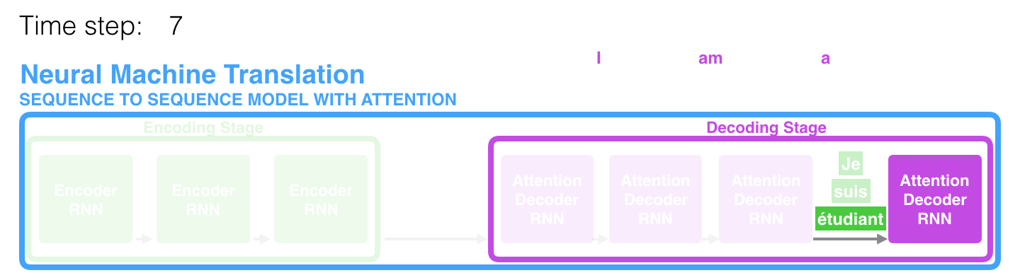
Bahdanau et al. (2014) proposed the attention mechanism: instead of relying solely on the final hidden state, the Decoder can look back at all of the Encoder's hidden states at each step.
Seq2Seq:           Encoder → c (a single fixed vector) → Decoder

Seq2Seq+Attention: Encoder → h₁, h₂, ..., hₜ (all hidden states)
                                    ↑ ↑ ↑
                                  Decoder dynamically selects which to attend to at each step
See the Attention mechanism notes for details.
Applications
Machine Translation (Core Application)
Seq2Seq was originally designed for translation tasks. In 2016, Google deployed its NMT system (based on Seq2Seq + Attention) in production, replacing its decade-old statistical machine translation system and achieving a dramatic improvement in translation quality.
Abstractive Summarization
Encoder input: a long article (potentially hundreds of words)
Decoder output: a concise summary (tens of words)
Unlike extractive summarization (which selects sentences directly from the source text), Seq2Seq can generate sentences not present in the original text, more closely resembling how humans write summaries.
Dialogue Systems
Encoder input: user's question "明天北京天气怎么样?"
Decoder output: system's response "明天北京晴,最高气温25度"
Early neural dialogue models (such as Google's Smart Reply) were built on Seq2Seq.
Speech Recognition
Encoder input: a sequence of audio features (e.g., mel spectrograms, potentially thousands of frames)
Decoder output: text "今天天气真好"
The vast difference in length between input and output is a perfect fit for Seq2Seq's design.
Historical Significance and Limitations of Seq2Seq
| Contribution | Description |
|---|---|
| Pioneered the Encoder-Decoder paradigm | This paradigm was directly inherited by the Transformer (the architecture in "Attention is All You Need" is still Encoder-Decoder) |
| Demonstrated the feasibility of end-to-end learning | No need to hand-craft translation rules; the model learns directly from data |
| Gave rise to the Attention mechanism | The fixed-vector bottleneck directly motivated the proposal of Bahdanau Attention |
| Limitation | Cause | Subsequent Solution |
|---|---|---|
| Fixed-vector bottleneck | All information compressed into a single vector | Attention mechanism |
| Sequential processing, no parallelism | Serial dependency of LSTMs | Transformer |
| Exposure Bias | Side effect of Teacher Forcing | Scheduled Sampling, RL-based training |
| Poor performance on long sentences | Bottleneck + LSTM's inherent memory limitations | Attention + Transformer |
Technological evolution:
Next: → Attention Mechanism (detailed mathematical principles of Attention) → Transformer Architecture