Adversarial Attack

Adversarial Attack refers to the technique in which a malicious attacker applies small, often imperceptible perturbations to input data, inducing machine learning models (especially deep neural networks) to produce incorrect outputs (such as misclassification). For example, by manipulating the input, an AI model can be tricked into recognizing a cat as a dog.

Key Concepts and Common Categories

Constraints and L-Norms

The essence of adversarial attacks is to deceive AI without being detected by the human eye.

To quantify "whether changes are visible to the human eye," three norms are commonly used:

$L_\infty$ norm: Limits the maximum change to any single pixel (e.g., each pixel can be altered by at most 8 intensity levels). This is the most commonly used norm because it ensures that no part of the image appears conspicuously different.
$L_2$ norm: Limits the sum of squares (total energy) of all pixel changes. It allows larger changes to some pixels, as long as the overall modification remains small.
$L_0$ norm: Limits how many pixels can be modified (e.g., only 10 pixels in the entire image can be changed, but by any amount).

It is worth noting that norms themselves are not exclusive to adversarial attacks. However, in this context, $L_\infty$ has become the signature norm of adversarial attacks because its strict constraint on the maximum per-pixel change best aligns with the human visual system — as long as no single point looks conspicuous, the image appears unchanged overall.

Common Attack Categories

In the field of AI security, attacks are generally classified into two major categories based on the phase in which they occur:

Poisoning Attack: Occurs during the training phase. The attacker injects malicious data into the training dataset, thereby compromising the model's integrity.
Evasion Attack: Occurs during the inference (deployment) phase. The model is already trained, and the attacker manipulates the input data to deceive it.

Adversarial ML (Adversarial Machine Learning) is an interdisciplinary field at the intersection of ML and computer security. Traditional computer security is typically binary (e.g., password correct/incorrect, permission granted/denied), whereas machine learning is based on probability and statistics. Adversarial ML studies the novel vulnerabilities that emerge when these two domains collide. For instance, biometric authentication, network intrusion detection, and spam filtering are all scenarios that rely on ML algorithms while demanding high security. If an attacker can bypass a spam filter (evasion attack) by subtly tweaking the text features of a spam email (adversarial example), the system's security breaks down.

In the security domain, the principle of "know your enemy before you can defend" applies. Researchers must first develop powerful attack algorithms (such as FGSM, PGD, C&W), generate adversarial examples capable of fooling models, and only then design targeted defense mechanisms (such as Adversarial Training).

Common Threat Types

Adversarial examples manifest in various forms, and the specific form of attack depends on three key factors of the attacker:

Goals: What they want to achieve (e.g., causing misclassification, model failure, or privacy breaches).
- Untargeted: The attacker simply wants the model to classify incorrectly. In the autonomous driving scenario discussed above, any misclassification can pose a significant safety hazard.
- Targeted: The attacker wants the model to misclassify the input as a specific, predetermined label. The intent is obvious — for example, forcing spam to be classified as legitimate email, or making identity A be recognized as identity B.
Knowledge: The essence of machine learning stems from the mathematical properties of high-dimensional spaces and statistical learning. Conversely, whether the attacker understands the model's internal structure determines the severity of the threat. Threat models are generally categorized by the attacker's level of knowledge:
- White-box attack: The attacker has complete knowledge of the model (architecture, parameters, weights, gradients, etc.). This is like having the blueprints of a safe, enabling precise calculation of how to crack it. Common methods: FGSM, PGD.
- Black-box attack: The attacker knows nothing about the internals and can only observe inputs and outputs. Typically, the attacker "queries" the model (feeding it large amounts of data and observing responses) to train a "surrogate model," then exploits the transferability of adversarial examples to launch the attack.
- Grey-box attack: Falls between the two extremes — the attacker may know the architecture but not the parameters, or may know part of the training data distribution.
Capabilities: The extent of influence they can exert on the system (e.g., modifying training data vs. only modifying test inputs). Generally, the technical methods available to attackers include:
- Crafting adversarial inputs: The attacker can design specialized adversarial inputs based on the model's predictions and probability distributions.
- Data preparation: The attacker can collect or generate auxiliary data.
- Model training (querying and substitution): By repeatedly querying the target model on the auxiliary dataset, the attacker uses the feedback to train a local substitute model, also known as a surrogate model.
- Exploiting transferability: Using the surrogate model as a white-box proxy to craft adversarial examples, and leveraging the transferability of adversarial examples so that they also work on the original target model.

Let us first examine the main threat models, and then analyze attack methods and defense mechanisms from first principles.

Causative Attack

Causative Attack (also known as Poisoning Attack) is an attack that occurs during the training phase. The attacker attempts to learn about, influence, or directly corrupt the machine learning model itself.

The mechanism works as follows:

Input contamination: Malicious training data is mixed into the regular training data.
Model training: The model is trained on the poisoned dataset.
Outcome triggering: If the resulting model achieves the attacker's desired outcome, the model is considered poisoned.

Evasion Attack

Evasion Attack, also known as Exploratory Attack, is an attack that occurs during the testing/inference phase. The attacker does not tamper with the machine learning model itself, but instead crafts carefully designed inputs to induce the model to produce specific output results chosen by the attacker.

The typical process is as follows:

Try Sample: The attacker submits a sample to the existing model.
Desired Outcome?: The attacker checks whether the model's output meets the intended goal.
Iterative Loop (Derive New Sample):
- If the desired outcome is not achieved (No), the attacker derives and generates a new sample based on the feedback, and tries again.
- If the desired outcome is achieved (Yes), the attack succeeds, achieving evasion.

Unlike the poisoning attack discussed earlier, evasion attacks are akin to finding "vulnerabilities" or "backdoors" in the system. The model is healthy at training time, but the attacker exploits weaknesses in the model's decision boundary to cause errors on specific data (for example, making an autonomous driving system recognize a "STOP" sign as a "speed limit" sign).

Evasion Attack is the most common type of attack.

The working principle of a machine learning classifier is to find a "boundary" between features of different classes. For example, suppose we are running an online auction website. To prevent users from selling prohibited items, we often train a Deep Convolutional Neural Network as an image classifier to distinguish "prohibited items" from "legitimate items."

As shown in the figure below, a classifier essentially separates different regions using a decision boundary:

1770984154963

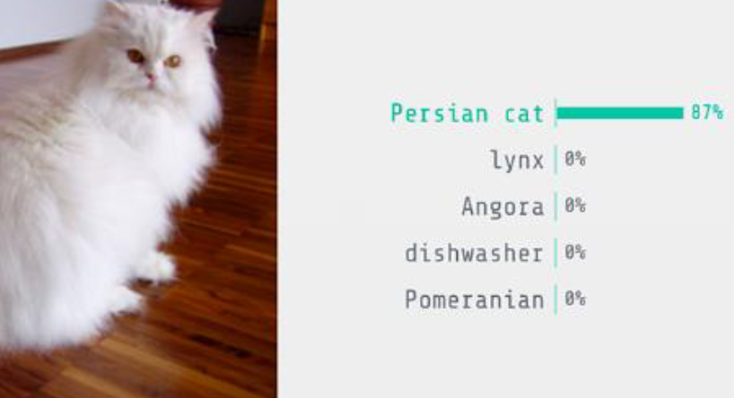
At its core, each image's pixels are converted into a vector, and the decision boundary is found in vector space. Since each image consists of tens of thousands of pixels, we have tens of thousands of variables that can be fine-tuned. By making extremely subtle adjustments to these pixels, we can push the image across the classifier's decision boundary.

As shown below, the modified image is identified by the same model as a toaster:

1770984166507

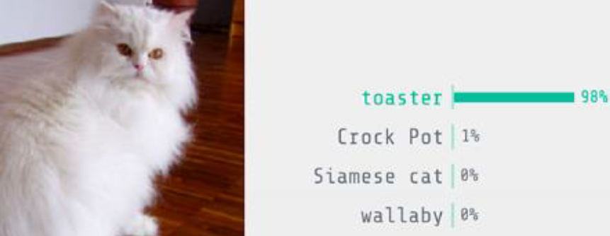
To the human eye, the modified image appears unchanged. But to the AI model, the same cat image is classified as a toaster with 98% confidence.

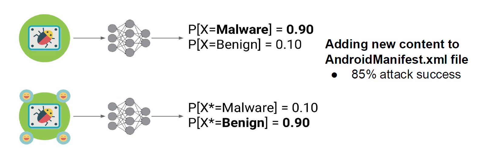
Evasion attacks are not limited to modifying image recognition results. Using the same methods, attackers can bypass the decision boundaries of any machine learning model to varying degrees, thereby achieving different malicious objectives.

As shown below, malware detection models can typically identify a file as malware with high probability. However, after the attacker adds some "inconsequential" new content to the AndroidManifest.xml file, even though the file's core malicious functionality remains unchanged, the model's judgment reverses — it now classifies the file as benign with 90% probability. This attack achieves a success rate of 85%, allowing malware to bypass detection and ultimately compromise systems.

1770984474509

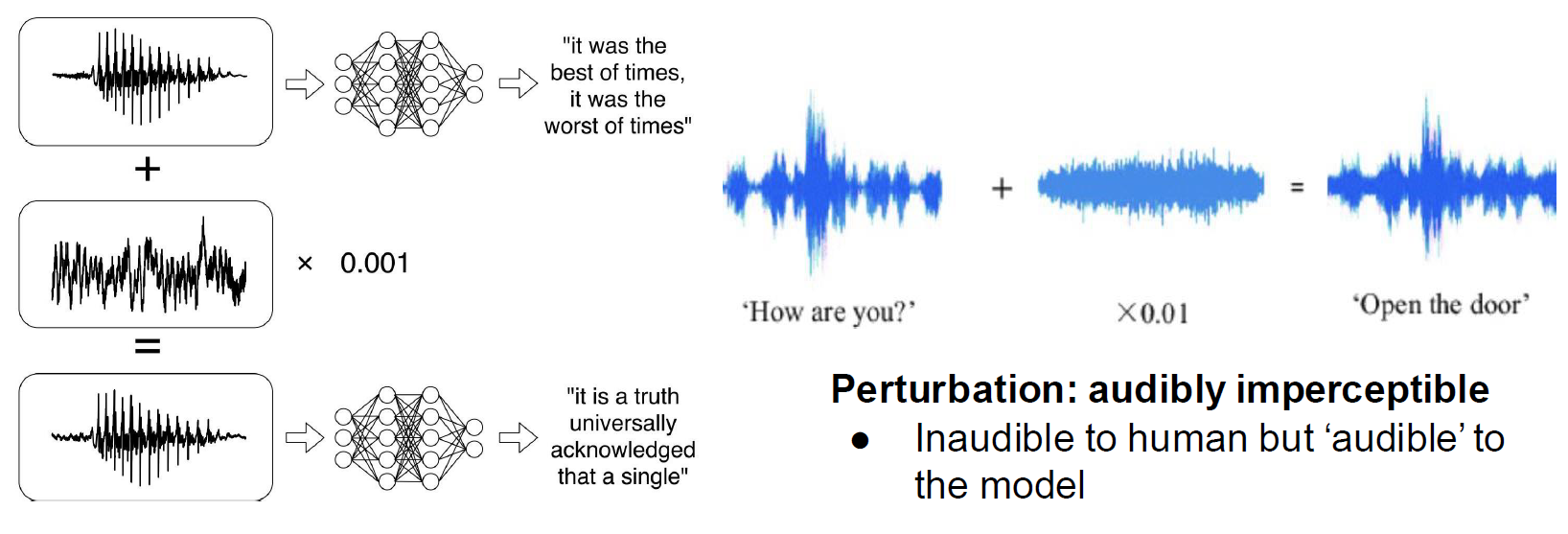
The same applies to speech recognition tasks. The attacker adds extremely small noise to the original audio (e.g., multiplied by a coefficient of $0.001$ or $0.01$). This type of disturbance is known as perturbation in adversarial attacks. Even though this noise is inaudible to humans, it constitutes "clearly visible" instructions for the AI model.

As shown below, through tiny perturbations, the attacker causes the model to misrecognize a literary quote about "the best/worst of times" as the opening of Pride and Prejudice, and tampers with the simple greeting "How are you?" into the highly dangerous command "Open the door." Such misrecognition could directly lead to safety hazards or physical harm (e.g., allowing an intruder into a home).

1770984580400

Adversarial attacks do not exist solely in the digital world — they can also infiltrate the physical world, since our real world is now highly integrated with information technology. For instance, many autonomous vehicles are now on the road, and they rely primarily on visual recognition to assess traffic conditions.

The figure below shows how attackers can subtly modify real-world traffic signs to induce AI model misclassification:

1770984782205

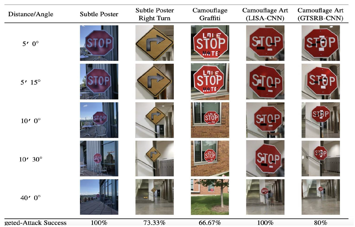
Attackers employed methods such as "Subtle Poster," "Camouflage Graffiti," and "Camouflage Art." Experimental results show that these modified "STOP" or "right turn" signs achieved extremely high attack success rates at various distances and angles. For example, certain "Subtle Poster" attacks achieved a 100% success rate. Such misrecognition can lead to severe consequences, such as traffic accidents.

The figure below illustrates an attack targeting the perception layer (lane line detection) of autonomous driving systems:

1770984860706

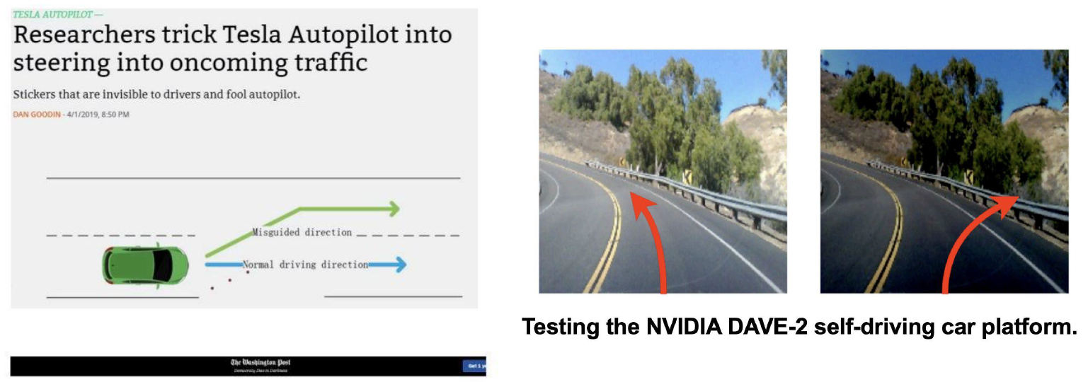
Researchers placed stickers on the ground that are nearly invisible to human drivers but capable of misleading the Autopilot system, inducing the vehicle to drive into the oncoming lane. The right side of the figure shows tests on the NVIDIA autonomous driving platform. Through specific perturbations, the system may fail to correctly identify lane boundaries or driving direction (the red arrows indicate the misled steering trajectory). Such misdetection can similarly result in safety hazards or direct physical harm.

These seemingly minor physical modifications can bypass AI defenses, transforming recognition/detection errors into physical harm in the real world.

We must rigorously consider the robustness of AI technology to ensure its reliability. Perturbations do not necessarily come from deliberate attacks. Since training sets cannot cover all possible situations, real-world unpredictability often produces unexpected results.

As shown below, Science & Diplomacy magazine discussed the challenges facing autonomous weapons:

1770985003093

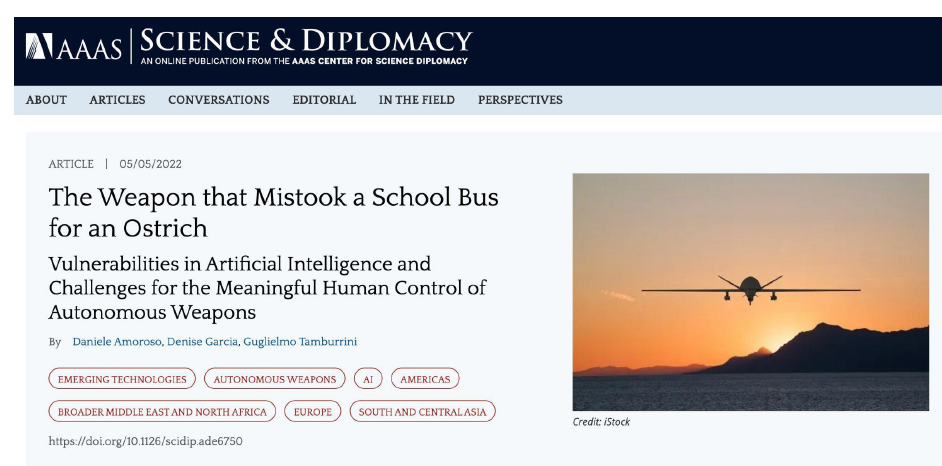
The article mentions an extreme misrecognition scenario in which a weapon might misidentify a school bus as a military convoy. This type of AI vulnerability could result in civilian casualties, raising serious international law and ethical concerns.

References:

2013: Szegedy et al., link: https://arxiv.org/abs/1312.6199, viewpoint: existence of low-probability nonlinear "pockets" and insufficient regularization.
2014: Goodfellow et al., link: https://arxiv.org/abs/1412.6572, viewpoint: the piecewise linear nature of DNNs (e.g., ReLU/Sigmoid) causes perturbations to be amplified.
2016: Tanay and Griffin, link: https://arxiv.org/abs/1608.07690, viewpoint: tilted decision boundaries prevent perfect model fitting.
2018: Schmidt et al., link: https://arxiv.org/abs/1804.11285, viewpoint: insufficient training data to guarantee robustness.
2018: Bubeck et al., link: https://arxiv.org/abs/1805.10204, viewpoint: constructing robust classifiers is computationally infeasible.
2019: Ilya et al., link: https://arxiv.org/abs/1905.02175, viewpoint: adversarial examples arise because models capture non-robust features.
2022: Amich and Eshete, link: https://arxiv.org/pdf/2202.08944.pdf, viewpoint: most adversarial examples are essentially out-of-distribution (OOD) inputs.

Privacy Attacks

Privacy attacks aim to extract sensitive information from the model's internals or training data. They fall into two main categories:

Model Inversion Attack: Uses the model's outputs and the model itself to reverse-engineer private and sensitive input data.
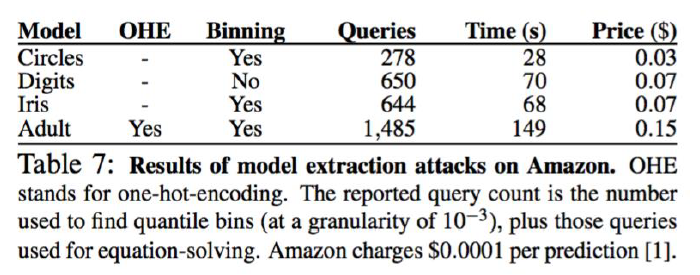
Model Extraction Attack: "Steals" or extracts the model's internal parameters by sending a large number of queries to the model.

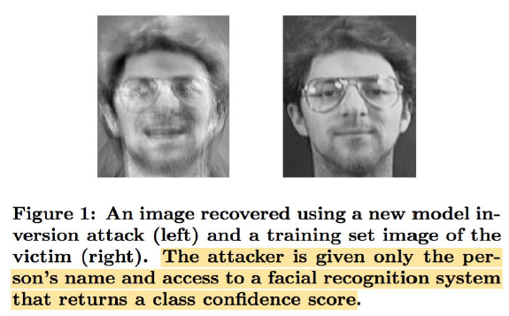
The figure below shows how confidence scores from a facial recognition system can be used to successfully reconstruct the victim's face:

1770985693979

The figure below demonstrates that the cost of conducting such attacks on platforms like Amazon is extremely low (e.g., only $0.03 to $0.15 per extraction):

1770985699495

White-Box Evasion Attacks on Images

Let us first discuss the most common type: white-box attacks.

Given a function $F: X \mapsto Y$ (which can be Logistic Regression, SVM, or a Deep Neural Network), the goal is to construct an adversarial sample $X^*$ by adding a perturbation vector $\delta_X$ to the original input $X$.

A white-box attack means the attacker has complete knowledge of the target model $F$ — the model architecture (e.g., ResNet, VGG), all parameters (weights and biases), and the training data distribution. Most critically, the attacker can access the model's gradient information, which is fundamental for generating adversarial examples via backpropagation.

Evasion means the attack occurs during the inference phase, after the model has been trained. The attacker does not alter model parameters through data poisoning, but instead deceives the model by modifying input data.

For example, in a CNN image recognition task: $X$ is the original pixel matrix (e.g., a photo of a panda), $Y$ is the probability vector output by the model (Softmax layer output), and $\delta_X$ is a carefully crafted noise pattern — not random noise, but specific noise computed with respect to model $F$'s decision boundary.

From this, we can write the mathematical definition of a white-box evasion attack:

\[ \arg \min_{\delta_X} \|\delta_X\| \quad \text{s.t.} \quad F(X + \delta_X) = Y^* \]

where $X^* = X + \delta_X$, and $Y^*$ is the adversarial output desired by the attacker (Targeted Attack).

This is clearly a constrained optimization problem:

Objective function $\min \|\delta_X\|$*: We want to minimize the perturbation. Visually, this means the adversarial sample *$X^*$ should be indistinguishable from the original sample $X$ to the human eye (imperceptibility). This distance is typically measured using $L_0, L_2, L_\infty$ norms.
Constraint $F(X + \delta_X) = Y^*$*: This is the condition for a successful attack. For example, the input originally classified as "panda" must now be classified as "gibbon" (*$Y^*$).
Intuitive understanding: We are searching for a "shortcut" in the high-dimensional feature space toward the target class $Y^*$, while requiring this shortcut to have the shortest physical distance.

When $F$ is nonlinear and/or nonconvex, solving this problem is non-trivial. Direct analytical solutions to the above optimization problem are impossible, so we must rely on approximate solutions.

JSMA

Let us examine the most fundamental algorithm: JSMA. This is a very early algorithm that we use to understand the basic idea, but note that it is completely impractical today. The specific reasons are explained at the end.

First, let us review the model training process using SGD as an example:

Fixed: The input data $X$ (e.g., an image of a cat).
Variable: The model weights $W$.
Objective: Compute the gradient $\nabla_W L$ of the loss function $L$ with respect to weights $W$, then update $W$ to minimize the loss.

During an attack, we reverse the logic:

Fixed: The model weights $W$ (the model is already trained; you cannot modify parameters).
Variable: The input data $X$ (you want to modify the image).
Objective: Compute the gradient $\nabla_X F$ of the output probability $F(X)$ with respect to input $X$, then modify $X$ to increase the probability of the target class.

In other words, during model training, we keep the image fixed and adjust the weights so the model can recognize the image; during an attack, we keep the weights fixed and modify the image so the model fails to recognize it.

JSMA (Jacobian-based Saliency Map Attack) uses a "saliency map" computed from the Jacobian matrix to find those few critical pixels that have the greatest impact on the result while being fewest in number. It does not care about all pixels — only those few "Achilles' heels."

Put differently, in standard SGD we compute $\frac{\partial Loss}{\partial W}$; in JSMA, we need to compute $\frac{\partial \text{class probability}}{\partial \text{pixel}}$.

We can first assess the sensitivity of model $F$ at input point $X$:

\[ \nabla F(X) = \frac{\partial F(X)}{\partial X} = \left[ \frac{\partial F_j(X)}{\partial x_i} \right]_{i \in 1..M, j \in 1..N} \]

This is essentially the Jacobian matrix. Suppose the input image has $N$ pixels and the model output has $M$ classes. The element $\frac{\partial F_j(X)}{\partial x_i}$ tells us: if we slightly change the value of pixel $i$, how much will the predicted probability of class $j$ change? In deep learning, we can efficiently compute this matrix by fixing the model parameters and performing backpropagation with respect to input $X$.

We can then select those perturbations that influence the classification of sample $X$. With the Jacobian matrix in hand, the attacker can construct a "heat map." For example, the attacker can identify pixels that have a high positive gradient for the target class $Y^*$ (increasing that pixel causes the target class probability to surge) and a high negative gradient for the original correct class (increasing that pixel causes the original class probability to plummet). By modifying only these critical pixels, the attack can be achieved with minimal perturbation ($L_0$ norm minimization).

For example, suppose the input is a $28 \times 28$ handwritten digit image (784 pixels total), and the model outputs probabilities for $0 \sim 9$ (10 classes).

SGD examines: The gradient of the loss with respect to millions of parameters.
JSMA examines: The gradient of the 10 class probabilities with respect to 784 pixels.

The matrix $J$ looks like this ($10$ rows $\times$ $784$ columns):

\[ J(X) = \begin{bmatrix} \frac{\partial \text{类0概率}}{\partial \text{像素1}} & \dots & \frac{\partial \text{类0概率}}{\partial \text{像素784}} \\ \vdots & \ddots & \vdots \\ \frac{\partial \text{类9概率}}{\partial \text{像素1}} & \dots & \frac{\partial \text{类9概率}}{\partial \text{像素784}} \end{bmatrix} \]

We can use backpropagation, treating the input image $X$ as the "parameters" while keeping the model parameters fixed. By performing backpropagation from each output node (class 0, class 1, ...) back to the input layer, we obtain this matrix.

With this matrix, we now know how each class probability changes when each pixel undergoes a small modification. Therefore, JSMA targets a specific attack (Targeted Attack) — for instance, suppose the original image is "1" and the attack goal is to make the model believe it is "4." JSMA follows a minimalist aesthetic: achieve the goal with as few modifications as possible. Hence, JSMA is an $L_0$ norm optimization:

Visual effect: A few strange bright spots or noise points appear on the image, resembling dead pixels.
Drawback: Computationally expensive (computing the entire Jacobian matrix is slow) — like performing surgery in slow motion.

The detailed JSMA process is shown below:

1770988286520

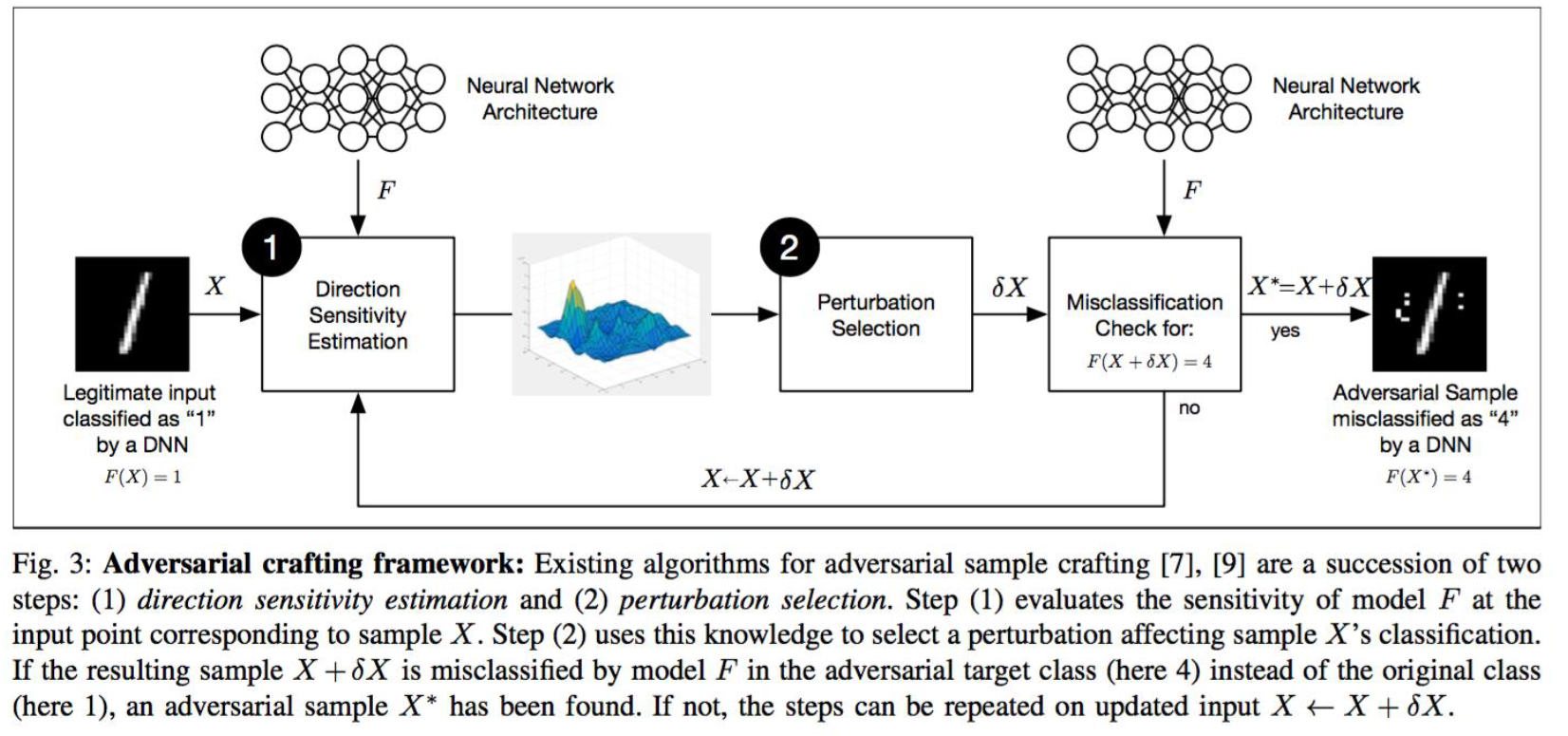
JSMA is an iterative, targeted white-box attack. Its core objective is: make the model misclassify digit "1" as "4," while modifying the fewest possible pixels ($L_0$ norm optimization). Following the flowchart above, we can roughly divide the entire JSMA process into four stages.

First, initialization and input:

Input ($X$): The left side of the flowchart shows an original handwritten digit "1" image.
Model ($F$): A trained deep neural network. Currently $F(X) = 1$ (correctly classified).
Attack target ($Y^*$): The attacker's specified target class $t = 4$.
Current state: The image is still the original; perturbation $\delta X = 0$.

Next, we perform Direction Sensitivity Estimation — this is the most critical first step in JSMA. Let us slow down and understand each term. Using the digit 1 from the diagram as an example, suppose you want to change it to digit "4" but can only modify a minimal number of pixels:

Direction: Refers to each specific pixel (e.g., the pixel at row 3, column 5). Mathematically, each pixel represents a "direction" along one dimension.
Sensitivity: Refers to how much the model's output probability of "this is digit 4" would fluctuate if you changed that pixel's value (e.g., from black to white).
Estimation: Because neural networks are too complex for direct computation, we must predict this change by computing derivatives (gradients).

The mathematical essence of direction sensitivity estimation is computing the Jacobian matrix. Suppose input image $X$ has $N$ pixels ($x_1, \dots, x_N$), and the model's output layer has $M$ classes ($F_1, \dots, F_M$). We need to compute the Jacobian matrix $J_F(X)$:

\[ \nabla F(X) = \frac{\partial F(X)}{\partial X} = \left[ \frac{\partial F_j(X)}{\partial x_i} \right]_{i \in 1..N, j \in 1..M} \]

where

$\partial F_j(X)$: represents the predicted probability of the $j$-th class (e.g., "panda" or "gibbon").
$\partial x_i$: represents the $i$-th input pixel.

In this matrix, we focus on two key pieces of information:

Gradient of the target class: $\frac{\partial F_t(X)}{\partial x_i}$ (where $t=4$). This represents: if we increase the value of pixel $i$, how much will class "4"'s probability increase? (We want this value to be as large as possible.)
Sum of gradients of other classes: $\sum_{j \neq t} \frac{\partial F_j(X)}{\partial x_i}$. This represents: if we increase pixel $i$'s value, how will the total probability of all classes except "4" change? (We want this value to be as small as possible, i.e., the other classes' probabilities should decrease.)

The 3D peak plot in the flowchart is the raw data computed from the above gradients. The highest peaks indicate the positions where pixels are most sensitive to the model's decision — in other words, these are the attacker's "best points of attack." The attacker uses this map to select perturbation points and modify X accordingly.

With the above principles understood, we can now construct the saliency map and implement the perturbation. The core idea is that for each pixel $i$, we check whether it satisfies two conditions:

Boosting the target: If we increase the brightness of pixel $i$, does the probability of the target class (4) surge?
- Check the table: $\frac{\partial \text{class 4}}{\partial x_i} > 0$ and is large.
Suppressing alternatives: If we increase the brightness of pixel $i$, do the probabilities of all other classes (including the original correct class 1) plummet?
- Check the table: $\sum_{\text{other classes}} \frac{\partial \text{other classes}}{\partial x_i} < 0$ and is strongly negative.

JSMA's logic is: A pixel is selected only if it can both significantly increase the target class probability and significantly suppress the probabilities of other classes. Such pixels receive a high saliency score.

JSMA defines a saliency score $S(X, t)[i]$ to evaluate the attack value of the $i$-th pixel.

An ideal attack pixel $i$ must satisfy both conditions simultaneously:

Positive contribution: Increasing it causes the target class (4) probability to increase (as seen through the derivative: $\frac{\partial F_t(X)}{\partial x_i} > 0$).
Negative suppression: Increasing it causes the total probability of non-target classes (e.g., the original class 1) to decrease ($\sum_{j \neq t} \frac{\partial F_j(X)}{\partial x_i} < 0$).

If both conditions are met, we compute its score (typically the product of the two); otherwise, the score is set to 0.

We find the pixel (or pair of pixels) with the highest score across the entire image:

\[ i_{best} = \arg \max_{i} S(X, t)[i] \]

In this step, the algorithm locks onto that single most lethal pixel.

Finally, we complete the modification through iteration. Unlike FGSM (introduced later), JSMA proceeds step by step and does not modify all pixels at once.

The JSMA algorithm proceeds as follows:

Input: Original image $X$, target class $Y^*=4$.
Loop (until the attack succeeds or the modification limit is reached):
1. Forward: Feed the current image into the network and compute the prediction. If it is already "4," stop.
2. Backward: Compute the Jacobian matrix (the sensitivity of each pixel under the current image).
3. Selection: Based on the saliency map formula, find the pixel (or pair of pixels) with the highest score.
4. Perturb: Aggressively modify this pixel. * Note: This is not a small SGD-style step of $\eta=0.001$. JSMA typically saturates the pixel (e.g., setting it to pure white or pure black, or adding a very large value).
5. Lock: This pixel is now "used up" (already modified) and will not be considered in subsequent rounds.
Continue loop: Take the image with one modified pixel and return to step 1.

The reason for looping is that neural networks are nonlinear. When you change a black pixel in the upper-left corner to white, the model's understanding of the entire image shifts. What was previously deemed "important" (e.g., a pixel in the lower-right corner) may no longer be so. Therefore, after each pixel modification, the Jacobian matrix must be recomputed.

As we can see, JSMA requires knowing the specific contribution of every input point to every output class. This was feasible on early MNIST handwritten digit datasets, but in the ImageNet and ViT era, computing the Jacobian matrix is practically impossible and unrealistic.

Furthermore, JSMA's underlying assumption is a fixed number of classes. If a ViT uses classification outputs, JSMA is theoretically still applicable. However, in the LLM era, we more commonly output the probability distribution over the next token and seek descriptions of images. In such scenarios, JSMA is completely ineffective.

FGSM

Fast Gradient Sign Method (FGSM) follows a carpet-bombing approach: instead of computing a complex Jacobian matrix, it computes the gradient of the loss function. The question it asks is: "In which direction should the overall input move to most rapidly increase the model's error rate?" Then, regardless of which specific pixels are sensitive, it shifts all pixels one small step ($\epsilon$) in that adversarial direction. The core of the formula is the sign() function, meaning all pixels change by the same magnitude.

Perturbation form ($L_\infty$ norm): All pixels undergo small changes.

Visual effect: The entire image is covered with a faint layer of snow-like noise or background hum, resembling interference on an old television signal.
Advantage: Extremely fast. Only one backpropagation pass is needed — nearly as fast as normal model inference.

Core idea of FGSM:

Central concept: Since training a model follows the opposite direction of the gradient (to decrease the loss), an attack follows the same direction of the gradient (to increase the loss).
Characteristic: Only one step. Extremely fast, but the attack is relatively "coarse."

DeepFool

DeepFool's objective is not "the fastest mistake" but rather "the minimum-cost mistake." It conceptualizes the neural network's decision boundary as a wall. It computes the shortest perpendicular distance from the current point to this wall, then gently pushes the point across it. Because neural networks are nonlinear (the wall is curved), it needs to iterate several times (push a little, recalculate, push again) until the boundary is crossed.

Perturbation form ($L_2$ norm): The sum of squares of overall changes is minimized.

Visual effect: Its perturbation is typically the most visually imperceptible among the three, because it pursues the mathematically minimum distance.
Advantage: Produces high-quality adversarial examples (extremely small perturbation), and is commonly used to evaluate model robustness (i.e., what is the smallest push that can topple the model?).

PGD

As mentioned in the JSMA section, JSMA is ineffective in the LLM era. As models grow larger and we move into an era where fixed-class prediction is no longer the norm, we need to return to loss-based attacks, because regardless of model size, the loss is always a scalar:

\[ \text{Loss} = \text{CrossEntropy}(\text{Output}, \text{Target}) \]

Computing the gradient of a scalar with respect to the input costs approximately one backpropagation pass regardless of model size. This is $M$ times faster (where $M$ is the number of output classes) than computing the Jacobian matrix (the derivative of a vector with respect to a vector).

In academia and industry, if you want to prove your model is "secure," you typically must pass PGD attack testing. FGSM's "one-shot" approach is easily defended against (e.g., through adversarial training), but PGD's "relentless iterative" attack is extremely hard to defend.

PGD is currently the most standard and powerful white-box attack method. Madry et al. proved in 2018 that PGD is the optimal attack achievable using first-order gradient information.

The PGD algorithm is an enhanced version of FGSM, with the following key steps:

Take a small step in the gradient direction.
Check whether the $L$ norm constraint has been violated (e.g., $L_\infty \le 8$).
If violated, forcibly project back onto the boundary (this is the "Projected" in the name).
Repeat the above steps.

AutoAttack

Although PGD is strong, recent research has found that more complex or combined attacks are more comprehensive and harder to defend than standard PGD. AutoAttack is not a single attack but rather combines multiple strong attacks into an "automated" evaluation pipeline, including:

Auto-PGD (with multiple loss functions)
FAB (Fast Adaptive Boundary)
Square Attack (can serve as a black-box component)

Overall, it generates adversarial examples that are more destructive than those from a single PGD attack, and it evaluates model robustness more reliably. Therefore, in modern evaluation, AutoAttack has become a more comprehensive white-box attack benchmark than PGD.

C&W Attack (Carlini & Wagner Attack)

The C&W attack, proposed by Carlini and Wagner in 2017, is one of the strongest optimization-based white-box attacks to date. It can effectively break through defenses such as distillation-based defense that were popular at the time.

Core idea: Transform the adversarial example generation problem into an unconstrained optimization problem. Introduce the variable substitution $\delta = \frac{1}{2}(\tanh(w) + 1) - x$, which naturally encodes the $L_\infty$ constraint into the variable space, thereby avoiding explicit projection operations. The objective function is:

\[ \min_w \|\delta\|_p + c \cdot f(x + \delta) \]

where $f$ is a specially designed confidence loss function (rather than directly using cross-entropy), and $c$ is a trade-off coefficient determined via binary search.

C&W $L_2$ Attack: The most commonly used variant, which minimizes the $L_2$ norm of the perturbation while satisfying the attack success constraint.

C&W $L_0$ Attack: The goal is to minimize the number of modified pixels (i.e., the $L_0$ norm). The algorithm employs an iterative pruning strategy:

First execute the $L_2$ attack to obtain an initial adversarial example.
Compute the gradient $g = \nabla f(x + \delta)$, and find the pixel with the smallest contribution to the classification result: $i = \arg\min_i g_i \cdot \delta_i$.
Remove pixel $i$ from the modifiable set (fix it to its original value).
Repeat the above process until the $L_2$ attack fails on the remaining pixels.

The final result is a minimal set of critical pixel perturbations that cause the classifier to err.

C&W $L_\infty$ Attack: The goal is to control the maximum perturbation magnitude (i.e., the $L_\infty$ norm). Since the $L_\infty$ norm is non-differentiable, an iterative penalty approximation strategy is employed:

\[ \min_\delta \; c \cdot f(x + \delta) + \sum_i \left[(\delta_i - \tau)^+\right] \]

where $(\cdot)^+ = \max(0, \cdot)$ denotes the ReLU function, and $\tau$ is the current maximum tolerated perturbation magnitude. The iteration rule is: if all $\delta_i < \tau$, then set $\tau := \tau \times 0.9$ (tighten the constraint); otherwise terminate. By progressively tightening $\tau$, the algorithm gradually converges to the true $L_\infty$ optimal solution.

Multimodal Visual Injection

Visual-GCG

Image-Hijack

White-Box Evasion Attacks on LLMs

White-box evasion attacks on LLMs are commonly referred to as jailbreak attacks in the LLM community.

GCG

GCG is one of the most prominent adversarial attack methods targeting large language models (LLMs), combining gradient search with discrete token substitution. It uses gradients to identify the token positions most likely to cause the model to produce undesirable outputs, then replaces the tokens at those positions. When GCG was proposed in 2023 (paper: Universal and Transferable Adversarial Attacks on Aligned Language Models), it caused enormous shockwaves because it demonstrated two alarming facts:

Universality: The nonsensical suffix it discovers is not only effective for "how to build a bomb" but also works for "how to steal credit cards" and "how to write a ransom note." It functions like a master key.
Transferability: Most alarmingly, an attack string computed on an open-source model (e.g., LLaMA) often remains effective when directly fed to closed-source models (e.g., ChatGPT, Claude, Bard). This means attackers do not need to know ChatGPT's parameters to attack it remotely.

AutoDAN

RepE, Activation Steering

This represents the most advanced level of white-box attack, at the "neurosurgery" level.

Core logic: Modern attackers have discovered that rather than painstakingly modifying the input (prompt), it is more effective to directly alter the model's intermediate states during reasoning.
The attacker identifies the neural activation direction representing "refusal" during model inference.
Operation: During inference, forcibly subtract the refusal direction (or add a "compliance" vector).
Why it is powerful: Dimensional superiority. As long as you have the model weights (white-box), this type of attack is virtually impossible to block with prompt-level defenses (such as system prompts), because you are directly modifying the model's "subconscious."

Loss Function Engineering

The goal goes beyond merely causing misclassification — it is about making the model err in a specifically designated way (e.g., recognizing a "cat" as "bread").

Untargeted Attack

Increase the $\text{CrossEntropy}$ by following the gradient, effectively "blinding" the model.

Targeted Attack (Altering Meaning)

Decrease $\mathcal{L}_{target}$ (e.g., for "dog"), precisely shifting the pixels toward the feature space of "dog."

Multimodal Injection

$\mathcal{L}_{desc}$ + $\mathcal{L}_{inj}$, balancing two forces: preserving the original meaning on one side while injecting malicious instructions on the other.

Transferability

After successfully attacking model A with PGD, can we continue to fool model B?

FOA / momentum terms / image transformations...

Black-Box Attacks

In black-box attacks, the attacker cannot access the target model's internal parameters or gradients and can only launch attacks by observing the model's input-output behavior. Based on the type of information available, black-box attacks are mainly divided into three categories.

Surrogate Model / Transfer-based Attack

Core idea: Since the target model is inaccessible, train a functionally similar "surrogate model," then perform white-box attacks on the surrogate and transfer the generated adversarial examples to the target model.

Papernot's Jacobian-based Dataset Augmentation (JBDA): Papernot et al. proposed a systematic procedure for training surrogate models:

Start with a small set of initial query samples, query the target model for labels, and construct an initial training set.
Train a surrogate model $\hat{F}$ on this dataset.
Use the surrogate model's Jacobian matrix $J_{\hat{F}}(x)$ to determine the most sensitive input directions, and perform dataset augmentation: generate new synthetic samples $x' = x + \lambda \cdot \text{sign}(J_{\hat{F}}(x))$.
Query the target model for labels on the new samples, add them to the training set, and iterate.

Finally, white-box attacks such as FGSM or PGD are applied to the surrogate model $\hat{F}$, and the resulting adversarial examples often successfully transfer to attack the target black-box model.

Transferability: If different models are trained on similar data, they tend to learn similar decision boundaries, causing adversarial examples generated on one model to be effective against another. Common techniques for enhancing transferability include: using ensemble models to generate attacks, introducing momentum terms, and applying random input transformations (Input Diversity).

Query-based Attack

The attacker estimates gradients by repeatedly submitting queries to the target model and observing outputs, then uses these estimates to generate adversarial examples. Based on the granularity of available output information, query-based attacks are further divided into two subcategories:

Score-based Attack: The target model returns the full probability vector (Softmax output). The attacker can estimate gradients using finite differences or Natural Evolution Strategy (NES):

\[ \hat{\nabla}_x \mathcal{L} \approx \frac{1}{n} \sum_{i=1}^{n} \frac{\mathcal{L}(x + \sigma u_i) - \mathcal{L}(x - \sigma u_i)}{2\sigma} u_i \]

where $u_i$ are randomly sampled directions and $\sigma$ is the smoothing parameter. A representative method is ZOO (Zeroth Order Optimization).

Decision-based Attack: The target model returns only the final prediction label (hard label), providing the least information and most closely resembling real-world deployment scenarios. Representative methods include Boundary Attack, which starts from a point that is already an adversarial example and walks along the decision boundary, gradually reducing the distance to the original image while maintaining attack success; and HopSkipJump Attack, which accelerates the search by estimating the gradient direction at the decision boundary.

Adversarial Defense

Adversarial Training

Adversarial training is currently recognized as the most effective adversarial defense method. Its core idea is to dynamically generate adversarial examples during training and incorporate them into the training set, forcing the model to learn feature representations that are robust to perturbations.

Min-max objective function:

\[ \min_{\theta} \max_{\epsilon:\|\epsilon\|_p \leq \sigma} \mathcal{L}(x + \epsilon;\, \theta) \]

The outer minimization (Min) corresponds to normal model training, optimizing parameters $\theta$; the inner maximization (Max) corresponds to the attacker's perspective, finding the perturbation $\epsilon$ that maximizes the loss under the $L_p$ norm constraint $\|\epsilon\|_p \leq \sigma$. This constitutes a two-player game: the attacker and defender compete during training, co-evolving together.

Equivalence with gradient regularization: It can be shown that adversarial training, under linear approximation, is equivalent to regularizing the gradient norm:

\[ \min_{\theta} \mathcal{L}(x) + \sigma \|\nabla_x \mathcal{L}\|_{p^*} \]

where $p^*$ is the dual norm of $p$ (satisfying $\frac{1}{p} + \frac{1}{p^*} = 1$). This means adversarial training smooths the gradient of the loss function, making the decision boundary flatter.

Main drawbacks: Adversarial training exhibits an accuracy-robustness tradeoff — improving robustness against adversarial examples typically leads to some decrease in standard accuracy on clean examples. Additionally, the computational overhead of adversarial training is significantly higher than standard training (requiring multiple steps of PGD attack within each batch).

Defensive Distillation

Papernot et al. proposed defensive distillation at IEEE S&P in 2016, which uses knowledge distillation techniques to smooth the model's decision surface in order to resist adversarial attacks.

Training procedure:

Train an initial classification network $F$ with temperature parameter $T > 1$ (high-temperature Softmax produces smoother probability distributions).
Use $F$ to generate soft labels $F(X)$ for the training set $X$; these soft labels contain inter-class similarity information.
Train the distilled network $F^d$ at the same temperature $T$ using the soft labels $F(X)$.

Defense mechanism: Training with soft labels makes $F^d$'s output probability distribution smoother with smaller gradient magnitudes, making it difficult for gradient-based attacks (such as FGSM) to find effective perturbation directions. Intuitively, the model's decision surface becomes "smoother," reducing sharp decision boundaries.

Limitations: Defensive distillation was later completely broken by Carlini and Wagner's C&W attack — the C&W attack specifically designed a new loss function targeting the Softmax layer, bypassing the gradient vanishing problem introduced by temperature scaling. This demonstrates that defenses relying on gradient obfuscation are fundamentally fragile.

Defense-GAN (ICLR 2018)

Defense-GAN uses a Generative Adversarial Network (GAN) generator to project input samples onto the data manifold learned by the model, thereby removing adversarial perturbations.

Core idea: Adversarial perturbations push inputs away from the true data manifold, and the GAN generator $G(z)$ precisely describes this manifold. Therefore, projecting the input back onto the manifold naturally eliminates the perturbation.

Algorithm: Given an input (possibly corrupted) image $x$, solve the following optimization problem:

\[ z^* = \arg\min_{z} \|G(z) - x\|^2 \]

Using $R$ random initialization points, each performing $L$ steps of gradient descent, select the $z^*$ with the minimum distance, and feed the "cleaned" image $G(z^*)$ into the classifier for prediction.

Limitations: The optimization process has high computational overhead; the choice of $L$ and $R$ affects the tradeoff between defense effectiveness and inference speed; strong adaptive attacks can incorporate the entire Defense-GAN pipeline into the attack objective.

Feature Squeezing

Feature squeezing removes potential adversarial perturbations by applying multiple transformations ("squeezers") to the input, and detects adversarial examples by comparing the prediction results between the original and squeezed inputs.

Common squeezing operations:

Bit-depth Reduction: Quantizes pixel values from 8-bit to lower bit depths (e.g., 4-bit or 2-bit), coarsening the feature space and eliminating fine-grained adversarial perturbations.
Spatial Smoothing: Applies median filtering or Gaussian blur to the image, eliminating local pixel-level perturbations.

Detection mechanism: If the model's prediction results for the original input $x$ and the squeezed input $\tilde{x}$ differ beyond a threshold, then $x$ is deemed an adversarial example and rejected.

\[ \text{If} \; \|F(x) - F(\tilde{x})\|_1 > \tau, \; \text{then reject input} \; x \]

Advantages: No model modification required; it serves as a plug-and-play preprocessing layer with low computational overhead. Limitations: Defense effectiveness drops significantly against adaptive attacks (where the attacker knows the squeezer exists).

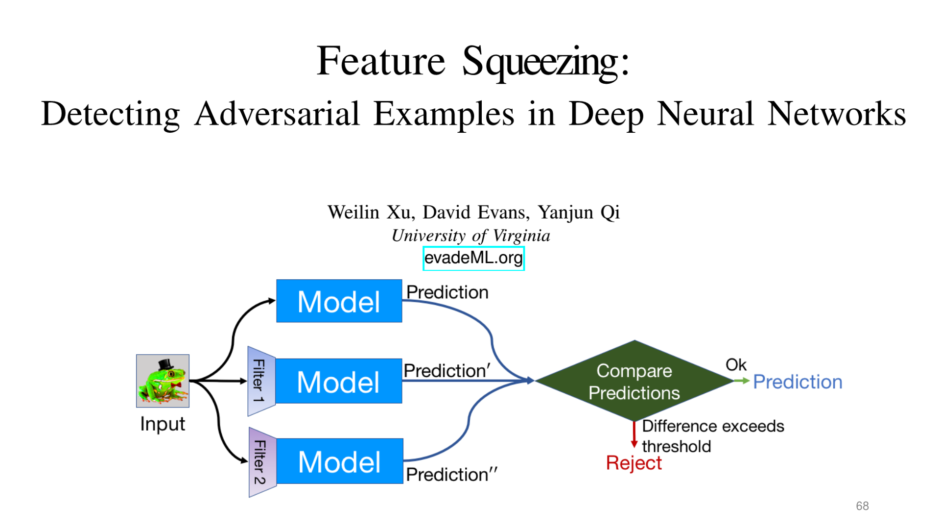
Feature Squeezing detection architecture

Source: Tufts EE141 Trusted AI, Lecture 3, Slide 68. Image note: three parallel inference paths compare prediction differences to detect adversarial inputs. Why it matters: the core idea of detection-based defense is forcing adversarial perturbations to produce inconsistencies across different representation spaces.

Adversarial Example Detection

Rather than correcting adversarial examples, an alternative defense strategy is to detect adversarial examples and reject them, allowing the system to deny service rather than make incorrect predictions.

Naive approach: Train a binary classifier to distinguish between original (normal) samples and adversarial examples. Input features can be raw pixels, intermediate layer activations, or statistical features (such as local pixel variance).

Main issues:

The detector itself can be attacked: Attackers can incorporate the detector into the attack objective, generating adversarial examples that simultaneously fool both the classifier and the detector (i.e., adaptive attacks). This is a "cat-and-mouse game" — introducing a detector only increases the attacker's cost but does not fundamentally solve the problem.
High computational overhead: Running the detector on every input introduces significant inference latency in real-time systems.
Poor generalization: Detectors trained on known attack types typically perform poorly in detecting unknown attack types (out-of-distribution attacks).

More mature detection methods: Statistical testing approaches (such as kernel density estimation, Mahalanobis distance) that detect distribution shifts in feature space, or leveraging model uncertainty (such as MC Dropout) to identify adversarial examples.