DQN
Reference code: cart_pole_v1
The DQN algorithm is a landmark achievement in reinforcement learning that directly triggered the explosion of Deep Reinforcement Learning (DRL). Before DQN, reinforcement learning primarily relied on table-based RL. Prior to DQN, researchers had been unable to find a suitable approximation method to replace these tables.
In 2013, DeepMind published the initial paper at NIPS, and in 2015 it was formally published in Nature. The core idea of DQN is: use a deep neural network (convolutional neural network) to replace the rigid Q-table.
DQN introduced three core mechanisms:
- Experience Replay
- Target Network
- End-to-End Learning
DeepMind used the same DQN algorithm and hyperparameters to surpass human expert players in most of 49 Atari games. This demonstrated that AI does not need task-specific hand-crafted rules, but instead possesses general learning capability. This directly pointed to the possibility of AGI and ushered in the era of "superhuman" AI.
The success of DQN directly gave rise to AlphaGo. Although AlphaGo later employed more advanced algorithms such as Policy Gradient, its underlying philosophy of "deep learning + reinforcement learning" was entirely inherited from DQN.
Q-Network
Q-Network
In traditional Q-learning, we maintain a Q-table where the horizontal axis represents actions and the vertical axis represents states. Take the classic CartPole task as an example: the states (position, velocity, angle, etc.) are continuous, so a table clearly cannot store them all.
Since there are infinitely many states, instead of recording specific values, we train a parameterized function \(Q_\omega(s, a)\) with parameters \(\omega\) to approximate the true Q-values. This function is implemented by a neural network, hence the name Q-network.
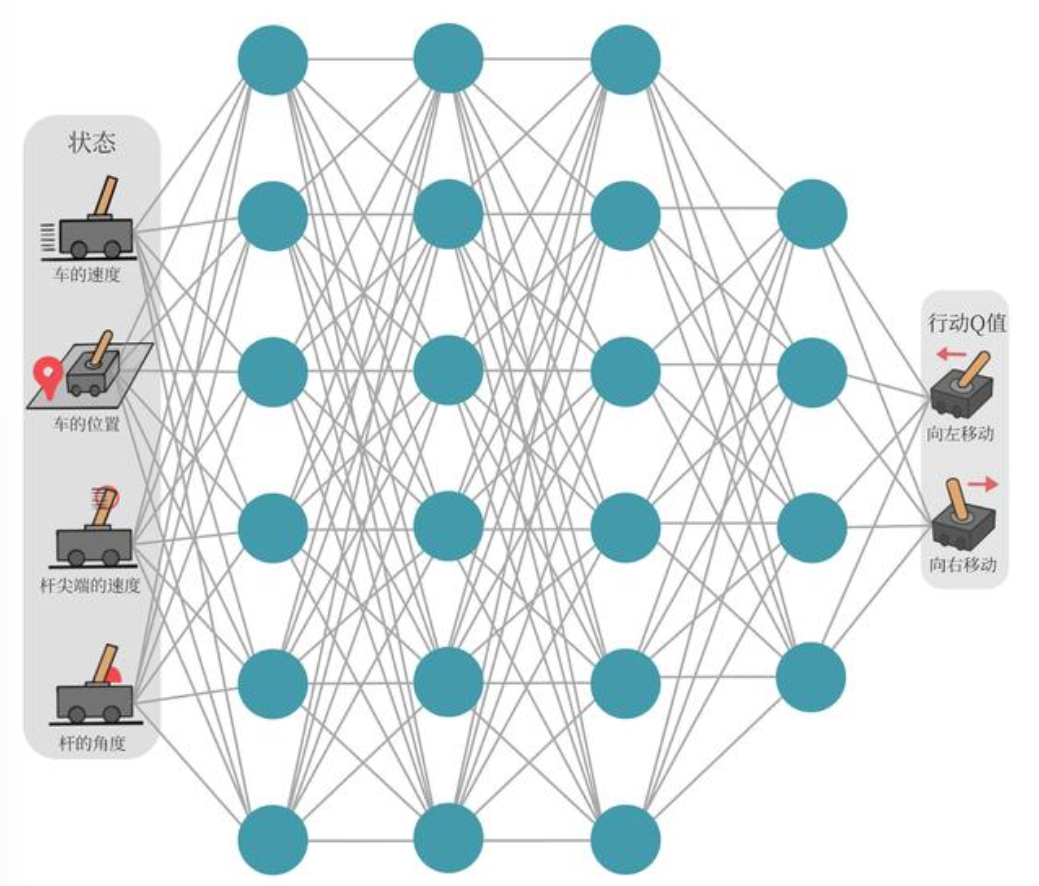
We can understand the Q-network from an input-output perspective:
- Input: State — e.g., game frames, CartPole state variables (angle, velocity, etc.)
- Hidden layers: e.g., a CNN architecture with convolutions, pooling, etc.
- Output: A vector — in the CartPole example above, the output consists of 2 neurons: move left or move right. The values of these two neurons represent the Q-values for taking each of these two actions in the current state.
The update rule of traditional Q-learning:
Where:
- \(r + \gamma \max_{a'} Q(s', a')\): This is the "ideal target" (TD Target) computed from the current reward and the best expected future return.
- \(Q(s, a)\): This is our current "subjective estimate."
- The learning rate \(\alpha\) drives our estimate closer to the ideal target over time.
When we replace the Q-table with a neural network \(Q_\omega\), the update rule becomes an optimization problem. In machine learning, the most common way to make one value approach another is through Mean Squared Error (MSE).
To make the neural network's prediction \(Q_\omega(s_i, a_i)\) approach the TD target, we construct the following loss function:
Where:
- \(Q_\omega(s_i, a_i)\): The current output of the neural network (predicted value).
- \(r_i + \gamma \max_{a'} Q_\omega(s'_i, a')\): The TD target (the benchmark we want the network to reach).
- \(\frac{1}{2N} \sum [... ]^2\): This is a standard MSE loss, and we use gradient descent to find the optimal parameters \(\omega^*\).
Although we now have a loss function, training the neural network directly is extremely unstable. Two key innovations that truly made DQN legendary:
- Experience Replay
- Target Network
Loss Function
Let us take another look at the loss function. In traditional deep learning (e.g., image classification), the loss function computes:
Here, the "ground truth" is pre-labeled by humans (e.g., this image is definitely a cat). But in reinforcement learning, we have no ground truth. How many points can the cart earn by pushing left in a certain state? No one tells the neural network in advance.
So how does DQN solve the problem of "no ground truth"? The answer is: use Q-learning's state transition logic to compute a relatively more accurate "ground truth" for itself.
The mapping between concepts can be broken down into three parts:
1. Network Prediction = "My current guess"
When the cart is in state \(s\) and is about to take action \(a\), the current neural network outputs a prediction: \(Q(s, a; \theta)\) (where \(\theta\) represents the network's current parameters).
- Physical meaning: This is the neural network's "pure guess" based on its current level of training.
2. Theoretical Target = "A more informed estimate with hindsight"
After the cart actually takes action \(a\), the environment provides a real immediate reward \(r\), and the cart enters the next state \(s'\).
According to the core of Q-learning (the Bellman optimality equation), given knowledge of the next state, the true value of the current action should be:
\(\text{Target} = r + \gamma \max_{a'} Q(s', a'; \theta^-)\)
- Physical meaning: Although this value still contains some guesswork (i.e., the estimated value of the next state \(\max Q(s', a')\)), it incorporates one piece of absolute ground truth from the environment — the immediate reward \(r\).
- Precisely because the real \(r\) serves as an anchor, and because we gain more information after taking a step, this Target value is necessarily closer to the truth than the purely speculative prediction \(Q(s, a; \theta)\). DQN treats it as the traditional "ground truth."
3. Loss Function = "Forcibly closing the gap between the two"
Now that we have a "current guess" (prediction) and a "more accurate guess" (target), the DQN loss function follows naturally: compute the Mean Squared Error (MSE) between them.
Therefore, we obtain the Loss:
Loss = Predicted value at state s - (actual reward from this step + discounted maximum predicted value at state s')
The formula is:
- The elegance of this combination: By feeding this difference to an optimizer (e.g., Adam), the neural network adjusts its parameters through backpropagation so that \(Q(s, a)\) on the left moves closer to the theoretical value on the right. With every environment interaction, we use new experiences from state transitions to correct the network's old, inaccurate Q-value estimates.
In summary: Q-learning's state transition logic is responsible for "manufacturing the correct target" (Target), while the loss function computes the deviation and, through the deep learning machinery, "drives the neural network's output to converge toward this target."
We must note that, since reinforcement learning has no ground truth, the real reward \(r\) is the only "anchor" in the entire formula. Suppose there were no real reward \(r\), and the target consisted only of \(Q(s', a')\). This would amount to requiring the network to make "the value of the current state" exactly equal to "the value of the next state." If trained this way, the laziest solution for the neural network would be: output Q-values of 0 for all states, instantly reducing the loss to 0! The cart would never learn to pursue a high score.
- \(Q(s, a)\) is pure guesswork.
- \(\max Q(s', a')\) is also guesswork.
- Only \(r\) is a hard fact provided by the environment.
Experience Replay
Reinforcement learning data is generated sequentially, with strong correlations between consecutive samples (e.g., when the pole is falling left, several consecutive samples all involve leftward tilting). This violates the independent and identically distributed (IID) assumption of machine learning. All neural network optimizers (e.g., Adam, SGD) rely on a strict mathematical assumption — the input data must be independently and identically distributed (i.i.d.). In other words, each batch fed to the network should ideally be randomly shuffled and mutually uncorrelated. When doing image classification, each batch contains cats, dogs, and cars, allowing the network to learn in a balanced manner.
Suppose the cart tilts rightward for 100 consecutive steps. If you immediately train the network on these 100 steps in real time, the neural network will severely overfit to the "tilting right" scenario, drastically adjusting its weights toward "push left aggressively." When the cart later tilts slightly to the left, the network has already "forgotten" how to handle left-tilting and crashes immediately.
The solution is to create a "buffer pool" that stores past experiences \(\{(s_i, a_i, r_i, s'_i)\}\), and randomly sample (shuffle) from it during training. This breaks the data correlation and improves efficiency. Specifically: store data into the pool, and during each training step, randomly sample a batch. This batch might contain data from step 5, step 100, left-tilting scenarios, right-tilting scenarios, etc. This forcibly transforms the temporally ordered reinforcement learning data into the "randomly shuffled dataset" that deep learning thrives on.
In cartpole_v1, the replay buffer stores nothing but pure physical objective facts, namely the five-tuple used in our code:
\((s, a, r, s', \text{done})\)
- \(s\): The screen at that moment (cart position, pole angle).
- \(a\): The decision made at that moment — push left or push right.
- \(r\): The score given by the environment on the spot.
- \(s'\): The state of the next frame after the push.
- \(\text{done}\): Whether the game ended at that moment.
The experience buffer is like a "ship's log" or a "dashcam recorder." It objectively records "at what point in time, what was on screen, whether you hit the gas or the brake, and whether there was a crash" — it contains no judgments of "right or wrong" or "value."
When we begin training:
- Randomly draw 64 "historical objective facts (log entries)" from the buffer.
- Feed these 64 historical states \(s\) as a batch to the current policy network (Policy Net). The network computes, via matrix multiplications and activation functions, its current predicted Q-values for these 64 states in real time.
- Feed these 64 historical next-states \(s'\) to the current target network (Target Net) to compute the target Q-values in real time.
We must never store Q-values in the experience buffer. Because the neural network is constantly evolving, old Q-values are outdated garbage.
Suppose in episode 1, the cart is a complete novice, and its Q-value estimate for state \(s_1\) is perhaps 0.1. This state is stored in the buffer. By episode 100, the cart has become an expert driver. When we draw \(s_1\) from the buffer again, we must not use the naive 0.1 from episode 1 as a reference. Instead, we feed the objective state \(s_1\) to the latest version of the neural network from episode 100 for a fresh evaluation. The current network takes a look: "Oh, this state is actually great — the Q-value should be 50!" This is the essence of why deep reinforcement learning works: using the latest brain (network weights \(\theta\)) to repeatedly review old memories (the \(s\) and \(s'\) in the replay buffer), thereby obtaining increasingly accurate understanding.
Experience replay also improves sample efficiency:
- The cart barely manages a spectacular "last-second save" at step 50, earning a critical reward. Without experience replay, the network computes one loss, slightly nudges its weights (limited by the tiny learning rate \(LR = 10^{-3}\)), and then discards this precious data forever.
- The replay buffer solution: This "last-second save" experience is stored in the buffer. Over the next few thousand training steps, it may be randomly sampled dozens of times. The neural network can thoroughly internalize the value of this action through repeated "review" of this critical memory, etching it into the DNA of its weights.
"A neural network is like an extremely lopsided student. If you let it study while doing homework (real-time input), it will forget algebra entirely after doing 10 geometry problems. The experience replay buffer is like building a problem bank (historical question set) for the student — each time, 64 randomly selected problems of different types are drawn for practice, ensuring well-rounded development."
Target Network
Let us revisit the Q-network's loss function:
Notice that both the "predicted value" on the left and the "target value" on the right contain the parameter \(\omega\). This is like taking an exam where every time you answer a question correctly, the answer key changes accordingly. How could you possibly pass?
Solution (Target Network):
- We clone two identical Q-networks: one called the "Online Network" and the other the "Target Network."
- When computing the loss, the target value on the right is computed by the "Target Network," whose parameters \(\omega^-\) are frozen.
- We only update the parameters \(\omega\) of the "Online Network" on the left.
- Every 1000 steps or at regular intervals, we synchronize the Online Network's parameters to the Target Network.
Let us develop a deeper understanding of why two networks are needed. Recall the DQN training process:
- Initialize a DQN network using a CNN architecture or any neural network architecture.
- Set up experience replay to store actual transitions.
- As the agent acts, after each step, sample a batch from the replay buffer to train the DQN: input the action-state pair, output Q-values, then compare the output Q-values against the actual values to compute the loss.
Here the problem arises: we have the output Q-values, but we have no actual values, because reinforcement learning has no labels — our data is all acquired through interaction with the environment. In RL, we call this actual value the target (Target). In RL, we have no Target and must construct one ourselves. This gives rise to the dual-network architecture mentioned above:
- Predicted Q — the DQN that first comes to mind, i.e., the policy network we are training.
- Target Q — the target network, which we deliberately set up to compute the loss.
How do we set up the target network? Since we need the Target to compute the loss, we obviously cannot set it up arbitrarily. There is an elegantly designed procedure (let us begin from when the replay buffer first fills a batch):
- At initialization, we create two identical networks called policy net and target net.
- When the replay buffer first fills a batch, we draw the first batch for training. We are always training the policy net — pay close attention to the following details.
- Suppose the first data point in the first batch is (s, a, r, s', not_goal), meaning:
state s, tookaction a (push right), received rewardr = 1 point, enterednext state s', game not over. - We feed state s to the policy net. The policy net performs a forward pass and computes the Q-value for action a (push right). This is called the predict Q. Since our policy net is still in its initialized state, let us assume this blindly guessed value is 0.5. This value is our predict Q.
- Next, we feed the next state s' to the target net. The target net examines s', and following the principle of Q-learning, we need to find the Q-value corresponding to the action with the maximum Q-value among all possible actions in state s'. Since the target net is also a novice at this point, let us assume it blindly guesses 0.8. We call this the next Q.
- Now we have two Q-values: predict Q and next Q. The former comes from s, the latter from s'. Now we need to construct the ground-truth label; otherwise we cannot compute the loss. We use the real reward r to fabricate the answer — r is the only real thing in the RL learning process. Suppose r = 1 here, then we fabricate the ground truth target Q = reward + gamma * next Q = 1 + gamma * 0.8. Assuming a discount factor gamma = 0.99, we get target Q = 1.792.
- Now we can compute the loss. loss = (target Q - predict Q)^2 = (1.792 - 0.5)^2
- Next, we perform backpropagation based on this loss to update the policy net's parameters. The objective is clear: the next time the network encounters \(s\), its output should shift from \(0.5\) toward \(1.792\).
- At this moment, something magical happens: the policy net's parameters have been modified — it has learned a tiny bit of experience about r = 1! However, we did not update the target net, so the target net remains completely unchanged.
However, we cannot freeze the target net forever. We typically set a synchronization period: within each period, the target net remains frozen; when the period elapses, we set target net = policy net, i.e., directly overwrite the target network's parameters with those of the policy network.
The Underlying Principle of Dual Networks
We now know that two networks are needed to construct the necessary components for computing the loss. But why can't we use just one network? In mathematics and optimization theory, this is known as the "Moving Target Problem." We can explain this by contrasting the mathematical essence of standard supervised learning with single-network Q-learning.
In standard supervised learning, when minimizing Mean Squared Error (MSE), the target value \(y\) is fixed (a constant).
If our neural network has parameters \(\theta\), and the prediction is \(f(x; \theta)\), then the loss function is:
When we differentiate with respect to \(\theta\) for gradient descent:
Because \(y\) is just a real label with no relation to \(\theta\), the direction of gradient descent is extremely stable and clear — simply converge toward \(y\).
If we use only one network, both Predict Q and Target Q are computed by the same network (with parameters \(\theta\)). The loss function we are optimizing becomes:
See the problem? Your target value \(Y(\theta)\) contains the very parameters \(\theta\) that you are updating.
When we perform gradient descent, attempting to adjust \(\theta\) so that Predict \(Q(s, a; \theta)\) approaches the Target, the Target \(Y(\theta)\) itself also shifts due to the change in \(\theta\).
In practice, Q-learning uses semi-gradient descent. When computing gradients, we forcibly ignore the target value's dependence on \(\theta\), pretending it is a constant.
But with a single network, this leads to severe instability:
- State \(s\) and next state \(s'\) are typically very close in feature space.
- When you update parameters \(\theta\) to increase \(Q(s, a)\), due to the generalization properties of neural networks, \(Q(s', a')\) typically increases in tandem.
- The result: you chase the target one step forward, and the target runs one step forward too. This creates a feedback loop where network weights can keep accumulating, ultimately causing \(Q\) values to diverge or oscillate wildly, making convergence impossible.
DeepMind introduced the Target Net in 2015, assigning a separate, frozen set of parameters \(\theta^{-}\).
With \(\theta^{-}\), the loss function becomes:
In this formula, the target value \(Y\) is computed entirely from \(\theta^{-}\). Because \(\theta^{-}\) is frozen (excluded from backpropagation) for a period of time, the target value \(Y\) mathematically becomes a true constant.
This temporarily reduces the unstable bootstrapping problem in reinforcement learning to a standard supervised learning problem. The network can comfortably fit toward a fixed target. Once the Policy Net has fit reasonably well, we hard-copy \(\theta\) to \(\theta^{-}\) (or perform a soft update), giving it a new fixed target for the next round of fitting.
Semi-Gradient Descent
Semi-gradient descent is where reinforcement learning (particularly TD-based algorithms) fundamentally diverges from traditional deep learning in its mathematical treatment.
In the ideal case, or in supervised learning tasks, we use full gradient descent.
Suppose we are doing a regression task where the prediction is \(V(S; \theta)\) and we have a perfect, fixed true target value \(U\). Our MSE loss function is:
If we differentiate with respect to \(\theta\) to update weights, the full gradient by the chain rule is:
This is perfectly sound — mathematically guaranteed that each update moves in the direction of decreasing loss.
In reinforcement learning (e.g., Q-learning or TD learning), we typically lack a "true" target value \(U\). Instead, we use bootstrapping — updating past estimates with current estimates.
In this case, our target value becomes \(R + \gamma V(S'; \theta)\). Notice that the target value also contains the parameter \(\theta\)****.
The true loss function then becomes:
If we were to compute the full gradient of this true function, the result would be:
See that \(-\gamma \nabla_\theta V(S'; \theta)\) at the end? That is the part arising from differentiating the target value with respect to \(\theta\).
In practical RL algorithms, computing that \(-\gamma \nabla_\theta V(S'; \theta)\) term is extremely difficult, and in many cases infeasible (because it involves the complexity of environment state transitions).
So the RL community made a simple, brute-force compromise: when computing gradients, pretend that the target value \(R + \gamma V(S'; \theta)\) is a constant, forcibly ignoring its dependence on \(\theta\).
This means we discard the gradient contributed by the target value and retain only the gradient from the prediction. The update rule becomes:
This is why it is called semi-gradient — because we only differentiated one half of the equation (the prediction part) and ignored the other half (the target part).
This mathematical "shortcut" has profound consequences:
- Advantage: Computational efficiency is greatly improved, enabling the algorithm to learn online through bootstrapping without needing to complete an entire episode before updating the network.
- Critical disadvantage: Because it is not true gradient descent, it loses convergence guarantees. It is like descending a mountain with a compass that only accounts for half the magnetic field — you will most likely veer off course.
This is also why there is a famous "Deadly Triad" theory in reinforcement learning: when function approximation (e.g., neural networks), bootstrapping (semi-gradient), and off-policy learning (e.g., Q-learning) all occur simultaneously, training is extremely prone to collapse.
Of course, in later improvements such as the PPO algorithm era, the use of on-policy methods resolved the Deadly Triad problem.
Training the Q-Network
Training Process
The pseudocode for the Q-network is as follows:
A plain-language walkthrough of the DQN process:
1. We use a CNN or any neural network architecture as the DQN. That is, we no longer store Q-values in a table; instead, we feed the state into the network to obtain Q-values.
※ Note: although the Q-function theoretically takes (s, a) as input, in practice we only input the state and output Q-values for all possible actions.
2. We set up an experience replay buffer to record actual cart trajectories.
3. Suppose episode = 500; each episode runs from the cart starting to move until it reaches the goal or hits the maximum episode step count.
4. Within each episode, we let the cart act and record: state, action, next state, reward, and whether the goal was reached.
5. We feed state s into the policy net to get predict Q. Note: we select the Q-value corresponding to the action the cart actually executed as the predict Q.
   We feed next state s' into the target net to get next Q. Following Q-learning, we take the action with the highest Q-value among all possible actions.
6. Using the actual reward r, we compute target Q. Then we compute the loss from target Q and predict Q, and use the loss to update the policy net's parameters.
7. We set a freeze period. When the freeze period elapses, we copy the policy net's weights to the target net.
8. During training, after each step the cart takes, we draw one batch for training. The first batch is drawn when the replay buffer first reaches one batch in size. The replay buffer operates as a FIFO queue.
.
Policy Collapse
Catastrophic Forgetting
Let us look at the results from programming/cart_pole_v1:
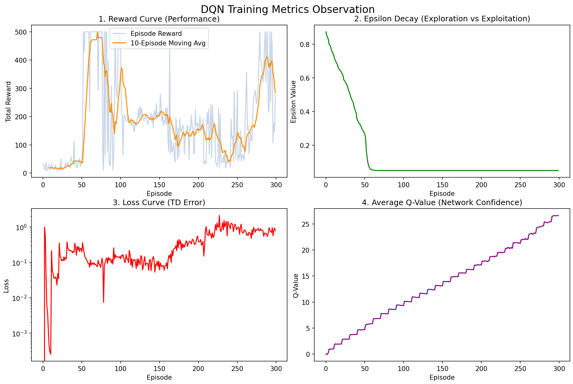
We can see that the reward already reached the maximum score between episodes 60-100, but then plummeted and oscillated between 100-200 points afterward.
We call this phenomenon policy collapse (Performance Collapse). Whenever your model was performing well and suddenly "goes stupid" — with scores plummeting and failing to recover — it can be called policy collapse. It is like saying a patient has gone into "shock": it describes a result, not the cause.
In this example, the cause of policy collapse is catastrophic forgetting. Because the experience replay buffer has limited capacity, when the cart maintains perfect balance for dozens of consecutive episodes, the buffer becomes filled with comfortable "how to go straight" data, while the earlier "how to recover from tilting" data gets pushed out. As a direct consequence, the network "forgets" how to handle crises. The moment a slight tilt occurs, it has no idea how to respond and collapses immediately.
Overestimation
Divergence due to overestimation is another common cause of policy collapse (and this is precisely the problem that DDQN aims to solve). The network's Q-value estimates for certain actions inflate like a balloon, eventually causing numerical explosion or promoting the wrong action to the top score. The network begins confidently executing extremely foolish actions (e.g., suddenly pushing the cart hard in a safe state, causing it to flip).
In PyTorch implementation, the core difference lies in just 1-2 lines of code for computing the target value (Target Q):
The blind confidence of vanilla DQN:
This is like having the "target network" serve as both the referee (evaluating how good actions are) and the athlete (selecting the highest-scoring action). Because it always picks its own perceived maximum, it is extremely susceptible to "overestimation."
In Double DQN, the target formula becomes:
This is like having the actively training "policy network" serve as the athlete to select the best action, and then having the frozen "target network" serve as the referee to score it. Even if the overconfident athlete picks the wrong action, the cool-headed referee will assign it a low score, thereby breaking the "overestimation" vicious cycle.
In cart_pole_v1, only one line of code needs to change:
# ==========================================
# 【原版 DQN 的代码】(既当运动员又当裁判)
# ==========================================
with torch.no_grad():
    # 直接用 target_net 选出最大值
    next_q_values = self.target_net(next_state_batch).max(1)[0].view(-1, 1)

# ==========================================
# 【修改为 Double DQN 的代码】(策略网络挑选,目标网络打分)
# ==========================================
with torch.no_grad():
    # 1. 策略网络 (policy_net) 挑出下一个状态的最优动作 (运动员)
    best_actions = self.policy_net(next_state_batch).max(1)[1].view(-1, 1)
    # 2. 目标网络 (target_net) 评估这个动作的价值 (裁判)
    next_q_values = self.target_net(next_state_batch).gather(1, best_actions)
It is that simple! When teaching, placing these two code snippets side by side instantly helps students understand the elegance of DDQN. For details, see the Double DQN section.
Double DQN
Target Q Improvement
In DQN, we have the following process:
A plain-language walkthrough of the DQN process:
1. We use a CNN or any neural network architecture as the DQN. That is, we no longer store Q-values in a table; instead, we feed the state into the network to obtain Q-values.
※ Note: although the Q-function theoretically takes (s, a) as input, in practice we only input the state and output Q-values for all possible actions.
2. We set up an experience replay buffer to record actual cart trajectories.
3. Suppose episode = 500; each episode runs from the cart starting to move until it reaches the goal or hits the maximum episode step count.
4. Within each episode, we let the cart act and record: state, action, next state, reward, and whether the goal was reached.
5. We feed state s into the policy net to get predict Q. Note: we select the Q-value corresponding to the action the cart actually executed as the predict Q.
   We feed next state s' into the target net to get next Q. Following Q-learning, we take the action with the highest Q-value among all possible actions.
6. Using the actual reward r, we compute target Q. Then we compute the loss from target Q and predict Q, and use the loss to update the policy net's parameters.
7. We set a freeze period. When the freeze period elapses, we copy the policy net's weights to the target net.
8. During training, after each step the cart takes, we draw one batch for training. The first batch is drawn when the replay buffer first reaches one batch in size. The replay buffer operates as a FIFO queue.
Specifically, step 5:
- We feed state s into the policy net to get predict Q. Note: we select the Q-value corresponding to the action the cart actually executed as the predict Q. We feed next state s' into the target net to get next Q. Following Q-learning, we take the action with the highest Q-value among all possible actions.
The only modification Double DQN makes is to step 5 above. The revised step 5 in Double DQN:
5'. We feed state s into the policy net to get predict Q. Note: we select the Q-value corresponding to the action the cart actually executed as the predict Q. We feed state s' into the policy net and select the action \(a^*\) with the highest Q-value; then we feed state s' into the target net and forcibly extract the Q-value corresponding to the previously selected \(a^*\) as the next Q.
The symbols involved in the above process are summarized as follows:
- \(r\): The real reward at the current step (Reward)
- \(\gamma\): Discount factor
- \(s'\): Next state
- \(a'\): Actions that may be taken in the next state
- \(\theta\): Parameters of the Policy Net (the network currently being trained)
- \(\theta^-\): Parameters of the Target Net (the frozen network)
The original DQN Target Q formula:
The Double DQN Target Q formula:
It is important to note that in the underlying theory of Markov Decision Processes (MDPs) and reinforcement learning, the absolute definition of the Q-function (Action-Value Function) is: the expected return from being in state \(s\), taking a specific action \(a\), and following the optimal policy thereafter. Since it evaluates a "state-action pair," it must mathematically be written as a function of two variables: \(Q(s, a)\).
However, in practice, for efficiency reasons, since the original DQN paper, the convention has been to input only the state and output Q-values for all possible actions. This way, regardless of how many actions there are, the neural network only needs one forward pass.
TD Error Optimization
When first learning DQN, we tend to use the phrase "make Predict Q converge toward Target Q" because it is very intuitive — like a shooting game where "the bullet (prediction) hits the bullseye (target)." But when you delve into classic top-venue RL papers or do production-level RL engineering at major companies, you will find that experts and papers almost exclusively discuss TD Error (\(\delta\)).
People often say "optimize the TD Error" because the loss function is constructed directly from the TD Error, so minimizing the TD Error is the ultimate optimization objective for the entire network update.
Here we distinguish between two concepts that share the same word "target" in some contexts:
- Target, i.e., TD Target: \(Y = r + \gamma \max_{a'} Q(s', a'; \theta^-)\)
- Objective, typically equivalent to the loss function:
The former is a concrete numerical value (the specific target value used when computing the TD error), while the latter is an action or task (the task of making the loss smaller).
In vanilla DQN, the experience replay buffer uses uniform sampling. But think about how humans learn: if you solve a problem and your prediction matches the answer perfectly (TD Error = 0), do you still need to review that problem? No. What you truly need to practice repeatedly are the problems where you were most wrong.
The absolute value of TD Error \(|\delta|\) physically represents the agent's "degree of surprise" or "learning potential."
- \(|\delta|\) is large: The gap between reality (Target) and expectation (Predict) is huge, meaning this data point contains enormous information, and we must sample it more frequently for training.
- \(|\delta|\) is near 0: We have already fully mastered this state; further training on it wastes compute.
Therefore, in the PER (Prioritized Experience Replay) algorithm, the TD Error magnitude directly determines the sampling probability of each data point in the replay buffer. Samples with larger TD Error are prioritized for training.
If you later study Actor-Critic methods (e.g., the PPO algorithm), you will encounter an extremely important concept called the Advantage function (\(A(s, a)\)). It measures "how much better is action \(a\) compared to what I would typically achieve by choosing blindly in this state?"
It can be mathematically proven that TD Error is actually an unbiased estimate of the Advantage function!
From this perspective, the entire optimization process of the Policy Gradient family is essentially following the direction indicated by the TD Error: increasing the probability of actions where \(\delta > 0\) (performance exceeded expectations).
Dueling DQN
Dueling DQN was proposed by the Google DeepMind team at ICML 2016 (International Conference on Machine Learning).
Value Stream Decomposition
In traditional DQN, regardless of the current state \(s\), the network must diligently evaluate the absolute value \(Q(s, a)\) for every action \(a\).
But in real life and games, there are many situations where "the choice of action simply does not matter":
- Scenario A (an open straightaway with no traffic ahead): You are in a very favorable state. Whether you accelerate, steer slightly left, or steer slightly right, the future return will be high regardless.
- Scenario B (a cliff ahead, brakes have failed): You are in a terrible state. Whether you honk, turn the steering wheel, or pull the handbrake, you will most likely go over the edge — the return for all actions is extremely low.
For traditional DQN, in Scenario B it must repeatedly learn: "honking scores -100," "turning the wheel scores -100," and so on. It wastes all its compute evaluating these "meaningless action differences" without astutely recognizing that it is the state itself that is terrible, regardless of which action is chosen!
To address this, Dueling DQN, in the final stage near the output layer, splits the original single fully connected layer into two parallel branches (this is the origin of the "Dueling" / "dual-stream" name):
- Value Stream — evaluating "how good is the state" Outputs a scalar \(V(s)\). Its physical meaning is: regardless of what action is taken next, how much is simply being in state \(s\) worth? (Similar to how Scenario B's base score is -100.)
- Advantage Stream — evaluating "how good is the action" Outputs a vector \(A(s, a)\) containing the advantage value for each action. Its physical meaning is: in this particular state, how much better or worse is action \(a\) compared to the average action? (It is a relative bonus.)
Finally, at the network's output, these two streams are added together to produce the final Q-value:
That is:
With this structure, if the network discovers that all actions yield the same result in a given state, it will simply learn \(V(s)\) accurately and drive all \(A(s, a)\) values to 0. This greatly improves the network's learning efficiency!
Unidentifiability
Suppose the network's final output \(Q\) value is 10.
- How did it get there? It could be \(V=10, A=0\).
- Or \(V=0, A=10\).
- Or even \(V=-100, A=110\).
Because there are infinitely many possible combinations of \(V\) and \(A\), the neural network during backpropagation becomes "confused," not knowing whether to update the \(V\) branch weights or the \(A\) branch weights, leading to extremely unstable training. This is "unidentifiability."
To force the network to treat \(V(s)\) as the true base score and \(A(s, a)\) as a purely relative advantage, the authors force the advantage stream to subtract its own mean at the aggregation step:
This way, the average of all actions' "advantages" is guaranteed to be 0.
Further Details
Q: How does the network learn "two types of value"? Does it have consciousness?
The network certainly has no consciousness. The reason it can learn \(V\) (state value) and \(A\) (action advantage) is entirely because it is forced to by "backpropagation (gradients)" and the "aggregation formula."
Let us look again at that masterful formula:
The network's loss is still computed by taking the final \(Q\) and computing MSE against the Target Q. The network does not "know" that the left component is called state value and the right component is called action advantage — it only knows it must reduce the loss.
Suppose in the current state, all 4 actions' Target Q values suddenly increase by 10 points uniformly. To reduce the loss, the network must increase its output across the board. The network has two options for updating its weights:
- Option A (the hard way): Modify the Advantage branch weights to increase \(A_1, A_2, A_3, A_4\) each by 10. But because the formula includes the "subtract the mean" operation, if all four actions increase by 10, the mean also increases by 10, and after subtraction it amounts to adding nothing! The gradient is largely canceled out here.
- Option B (the shortcut): Directly modify the Value branch weights to increase \(V(s)\) by 10. This operation encounters no resistance, is extremely efficient, and instantly reduces the loss.
Because of the "subtract the mean" constraint, the gradients from backpropagation automatically seek the path of least resistance. If the overall score rises, the gradient naturally flows to the \(V\) branch; if a particular action's score stands out, only then does the gradient flow to the \(A\) branch. This is the fascinating phenomenon of representation decoupling in deep learning.
Q: How do the two streams produce different outputs from the same input? (Physical structure and initialization)
We can visualize the forward pass logic in code:
- Shared Layers (Shared Representation):
The input state \(s\) (e.g., an image) first passes through several CNN layers for feature extraction. The last CNN layer outputs a 512-dimensional vector
feature_vector. Up to this point, everything shares the same set of weights. - Physical Branching:
This 512-dimensional vector is then simultaneously fed into two distinct fully connected layers. These two layers have different weight matrix dimensions!
- Value branch (evaluating the state): A linear layer of shape
[512, 1]. It compresses the 512 features into a single number (the \(V\) value). - Advantage branch (evaluating actions): If the environment has 4 actions, this is a linear layer of shape
[512, 4]. It maps the 512 features into 4 numbers (the \(A\) values for 4 actions).
- Value branch (evaluating the state): A linear layer of shape
As we can see, the outputs differ because:
- Different structure: One outputs 1 dimension, the other outputs 4 dimensions — the computation matrices are inherently different.
- Random initialization: At the start of training, the weight matrices and biases of both branches are randomly initialized. Even with the same 512-dimensional feature input, their initial outputs will certainly differ.
- Independent updates: During subsequent training, because the aggregation formula distributes gradients toward different tasks, these two sets of independent weights diverge completely. One set strives to fit the average base salary (\(V\)), while the other strives to fit the performance bonus (\(A\)).
Physically, they are two separate sets of independent network parameters; mathematically, they are given different starting points through random initialization; mechanistically, they are forced by the special aggregation formula to take on different semantic roles.