RNN Principles
Questions to think about:
- Why can't RNNs perform parallel computation?
- For an entire book, can an RNN really remember what was written in the first chapter?
- CNNs process images and RNNs process sequences — what are their respective inductive biases?
From MLP/CNN to RNN
Why Do We Need a New Architecture?
As we saw in the CNN principles notes, CNNs solve image processing problems through two core inductive biases (locality and translation invariance). However, data such as natural language, speech, and stock prices are sequences — elements have a temporal ordering, and the length is variable.
MLPs and CNNs have fundamental shortcomings when processing sequences:
| Architecture | Problem with Sequences |
|---|---|
| MLP | Fixed input dimensionality — "I like cats" has 3 words, while "the weather is nice today" has 5 words. MLPs cannot handle inputs of varying lengths. Forced padding is wasteful and destroys structure |
| CNN | Convolution kernels only see a fixed-size local window (e.g., 3x3). For long-range dependencies like "although the beginning was boring, the ending was brilliant" (where "although...but..." spans many words), CNNs need to stack a very large number of layers to cover such distances, which is extremely inefficient |
Core requirement: We need an architecture that can:
- Process input sequences of arbitrary length
- "Remember" previously seen content when processing the current element
- Share parameters across time steps (analogous to how CNNs share convolution kernels across spatial locations)
Core Inductive Biases of RNNs
By analogy with the analysis approach used in the CNN notes, RNNs also have two core inductive biases:
| CNN | RNN |
|---|---|
| Locality: a pixel is most closely related to its neighboring pixels | Temporal dependence: the output at the current time step depends primarily on the current input and historical information |
| Translation invariance: a cat in the top-left corner and the bottom-right corner is still a cat | Temporal translation invariance: the "rules" for processing the sequence are the same at every time step (parameter sharing) |
CNN parameter sharing is spatial (the same convolution kernel is used at different locations in the image), while RNN parameter sharing is temporal (the same set of weights is used at different time steps of the sequence).
Mathematical Foundations
Mathematical Derivation from MLP to RNN
Attempting to Process Sequences with an MLP
Suppose we want to process a sequence of length \(T\): \(x_1, x_2, \ldots, x_T\). The most naive approach is to concatenate all time steps and feed them into an MLP:
Problem: the size of \(W\) depends on \(T\), so sequences of different lengths require networks of different sizes. Moreover, each time step position is bound to specific weights, preventing generalization.
Introducing the Concept of "State"
What if, instead of looking at all inputs at once, we process them step by step? At each step, we maintain a "state" that summarizes the historical information:
This is the core idea behind RNNs: \(h_t\) (the hidden state) is a compressed summary of \(x_1, x_2, \ldots, x_t\).
Parameter Sharing
By analogy with the derivation in the CNN notes — CNNs achieve spatial parameter sharing by making the weights independent of position \((i,j)\). RNNs achieve temporal parameter sharing by making the weights independent of time step \(t\):
- Without sharing: \(h_t = f(W_t^{hh} \cdot h_{t-1} + W_t^{xh} \cdot x_t + b_t)\) (each time step has its own weights)
- With sharing: \(h_t = f(W^{hh} \cdot h_{t-1} + W^{xh} \cdot x_t + b)\) (all time steps use the same set of weights)
This allows RNNs to process sequences of arbitrary length, with a parameter count independent of sequence length.
Complete Formulation of Vanilla RNN
Hidden state update:
Output computation:
Notation:
| Symbol | Dimension | Meaning |
|---|---|---|
| \(x_t\) | \(\mathbb{R}^d\) | Input vector at time step \(t\) (e.g., a word embedding) |
| \(h_t\) | \(\mathbb{R}^{d_h}\) | Hidden state at time step \(t\) (a summary of historical information) |
| \(h_{t-1}\) | \(\mathbb{R}^{d_h}\) | Hidden state from the previous step |
| \(W_{xh}\) | \(\mathbb{R}^{d_h \times d}\) | Input-to-hidden weight matrix |
| \(W_{hh}\) | \(\mathbb{R}^{d_h \times d_h}\) | Hidden-to-hidden weight matrix (recurrent connection) |
| \(W_{hy}\) | \(\mathbb{R}^{d_o \times d_h}\) | Hidden-to-output weight matrix |
| \(b_h, b_y\) | Bias terms | |
| \(\tanh\) | Activation function (squashes values to \([-1, 1]\)) |
Parameter count analysis: Suppose \(d = 300\) (word embedding dimension), \(d_h = 256\) (hidden layer dimension), \(d_o = 10000\) (vocabulary size):
Note: regardless of how long the sequence is (10 words or 10,000 words), the parameter count remains 2.7M. This is the power of parameter sharing.
Architecture Details
Folded View vs. Unfolded View
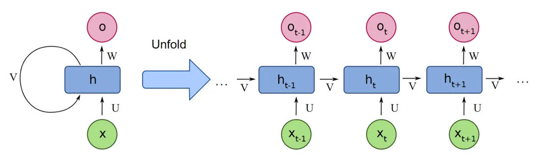
RNNs have two equivalent representations — the folded view and the unfolded view:
Meaning of Each Symbol in the Diagram
| Symbol | What It Represents | Analogy |
|---|---|---|
| \(x\) (green circle) | Input vector, e.g., a word embedding | Raw material |
| \(h\) (blue square) | Hidden state vector, e.g., \([0.48, -0.36, 0.72]\), a collection of numbers | Semi-finished product (can be further processed or shipped directly) |
| \(o\) (pink circle) | Output vector, the final result after transformation by \(W\) | Finished product |
| \(U\) | Input-to-hidden weight matrix (corresponds to \(W_{xh}\) in the formulas above) | Tool for processing raw materials |
| \(V\) | Hidden-to-hidden weight matrix (corresponds to \(W_{hh}\) in the formulas above) | Tool for leveraging past experience |
| \(W\) | Hidden-to-output weight matrix (corresponds to \(W_{hy}\) in the formulas above) | Tool for final inspection |
Symbol correspondence
Different textbooks use different letters. This diagram uses \(U, V, W\); the formulas above use \(W_{xh}, W_{hh}, W_{hy}\); Colah's Blog uses \(A\) to represent the entire computational unit. They all refer to the same thing — don't be confused by the different letters.
Folded View (Left Side)
The left side shows a structure with a self-loop:
- \(x\) enters \(h\) through weight \(U\)
- \(h\) outputs \(o\) through weight \(W\)
- \(h\) simultaneously feeds back into itself through weight \(V\) (the self-loop arrow)
This self-loop is the origin of the name "recurrent" neural network — the output of \(h\) is fed back to itself as input for the next time step.
Unfolded View (Right Side) — The Key Concept
Unfolding the self-loop along the time axis clearly reveals how information flows step by step:
Step-by-step reading:
- Time \(t-1\): Input \(x_{t-1}\) enters through \(U\), combines with the hidden state passed from the previous step → produces \(h_{t-1}\)
- \(h_{t-1}\) splits into two paths: - Upward: through \(W\) to output \(o_{t-1}\) (the prediction at this time step) - Rightward: through \(V\) to the next time step (this is the transmission of "memory")
- Time \(t\): \(h_{t-1}\) arrives from the left (through \(V\)), \(x_t\) arrives from below (through \(U\)), and together they determine \(h_t\)
- \(h_t\) again splits into two paths: upward to output \(o_t\), rightward to \(h_{t+1}\)
- Time \(t+1\): same process, and so on...
Corresponding Mathematical Formulas
The computation inside each blue square \(h\) in the diagram:
The computation for each pink circle \(o\):
Key insight: \(h_t\) is not a neuron but a vector (a collection of numbers). The blue square represents a computation process (matrix multiplication + tanh), and \(h_t\) is the output of that computation. \(h_t\) simultaneously plays two roles: (1) it passes upward through \(W\) to become the output \(o_t\); (2) it passes rightward through \(V\) to become the input for the next step.
All time steps share the same set of parameters \(U, V, W\) — this is RNN's parameter sharing, analogous to how CNN convolution kernels are shared across different spatial locations.
The unfolded view is the key to understanding RNNs: once unfolded, an RNN looks just like a very deep feedforward network, except that each "layer" shares the same weights. This is also why RNNs encounter gradient problems similar to those in deep networks.
Complete Forward Propagation Process
RNN forward propagation is simply standard matrix multiplication, fundamentally no different from a fully connected layer in an MLP. Using the sequence "I like cats" as an example (assuming \(d=4, d_h=3\)):
Initialization: \(h_0 = [0, 0, 0]\) (zero vector)
Step 1: Processing "I"
(a) Concatenation (or separate multiplication followed by addition — mathematically equivalent):
Expanding the matrix multiplication:
Since \(h_0 = \vec{0}\), the first term is zero, so:
(b) Activation:
That is the entirety of one RNN forward propagation step. It is simply one matrix multiplication + tanh.
Step 2: Processing "like"
Now \(h_1 \neq \vec{0}\), so \(W_{hh}\) comes into play:
The results of the two matrix multiplications are summed: \(W_{hh} \cdot h_1\) carries the memory of "I", while \(W_{xh} \cdot x_2\) brings in the new information from "like".
Step 3: Processing "cats" — exactly the same process, yielding \(h_3\).
Summary: RNN forward propagation = repeating the same fully connected layer at each time step (two matrix multiplications + one tanh), with the previous step's output serving as an additional input for the next step. There is nothing beyond basic forward propagation.
Hidden State Storage (Training vs. Inference)
During training: all intermediate hidden states \(h_0, h_1, h_2, h_3\) computed at each step are stored in memory and are not overwritten. This is because backpropagation requires all intermediate values to compute gradients. Therefore, the memory cost of RNN training is proportional to the sequence length — the longer the sequence, the more \(h\) values must be stored, and the greater the GPU memory consumption.
During inference: backpropagation is not needed, so only the latest \(h_t\) needs to be kept; previous \(h\) values can be discarded. This is why the memory cost of RNN inference is constant.
Computation Graph and "Why Parallelization Is Impossible"
The unfolded diagram makes it clear:
Computing \(h_2\) must wait for \(h_1\) to finish, and \(h_3\) must wait for \(h_2\) to finish. This is a strict sequential dependency chain — it cannot be parallelized.
By contrast, convolutions at different positions in a CNN can be computed simultaneously (there are no dependencies), and a Transformer's Self-Attention can process all positions at once. This is the fundamental reason why RNN training is slow.
| Architecture | Computing outputs at \(n\) positions | Number of sequential operations |
|---|---|---|
| RNN | Must proceed step by step | \(O(n)\) |
| CNN | All positions in parallel | \(O(1)\) (single layer) |
| Transformer | All positions in parallel | \(O(1)\) |
Backpropagation: BPTT
Backpropagation Through Time
RNNs are trained using Backpropagation Through Time (BPTT). The core idea: treat the unfolded RNN as an ordinary deep feedforward network and perform standard backpropagation.
Why can gradients propagate all the way from \(h_t\) back to \(h_0\)?
During forward propagation, all intermediate hidden states \(h_0, h_1, \ldots, h_t\) are stored in memory (see the explanation in the forward propagation section). During backpropagation, these stored values are used to compute gradients step by step from back to front. The \(h\) values are not "overwritten" — each \(h_t\) at every time step is an independently stored variable, not the same variable being repeatedly reassigned.
Suppose the loss function is the sum of losses at each time step:
We need to compute \(\frac{\partial \mathcal{L}}{\partial W_{hh}}\). Since \(W_{hh}\) is used at every time step, the gradient must be accumulated across all time steps:
For the loss \(\mathcal{L}_t\) at a particular time step \(t\), its gradient with respect to \(W_{hh}\) must be traced back through \(h_t, h_{t-1}, \ldots, h_1\):
The gradient traced from \(h_t\) back to \(h_k\) is a chain of products:
Vanishing Gradient and Exploding Gradient
The chain of products above is the root of the problem. The range of \(\tanh'(x)\) is \((0, 1]\), so each factor is at most 1.
Vanishing Gradient: When the largest singular value of \(W_{hh}\) is < 1:
Multiplying \(t - k\) factors, each less than 1 → exponential decay → gradients from early time steps approach zero.
The following diagram intuitively illustrates the BPTT process — black arrows represent forward propagation, red arrows represent gradient backpropagation, and you can see that gradients must travel all the way back along the time axis:
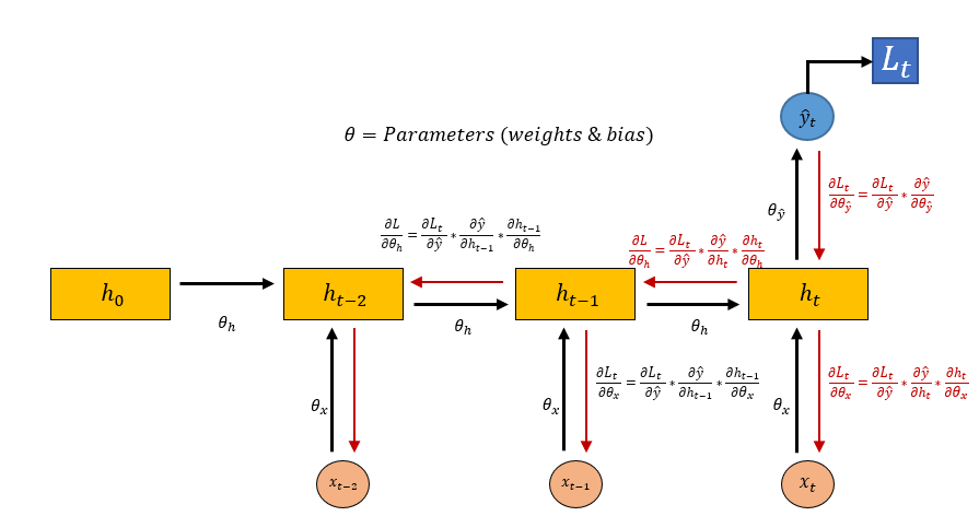
In the diagram, \(\theta_h\), \(\theta_x\), and \(\theta_{\hat{y}}\) correspond to the three weight matrices \(V\) (hidden-to-hidden), \(U\) (input-to-hidden), and \(W\) (hidden-to-output), respectively. As shown, the gradient of \(\theta_h\) must be chained from \(h_t\) all the way back through \(h_{t-2}\), \(h_{t-3}\), and so on. The longer the sequence, the more multiplications in the chain, and the more susceptible the gradient is to vanishing or exploding.
Intuitive understanding: when training the model to process "although the beginning was boring the ending was brilliant", \(\mathcal{L}\) comes from the prediction at the last step "brilliant". The gradient must propagate all the way back from "brilliant" to "although", and after 5 chained multiplications it is nearly zero. The model fails to learn the contrastive relationship "although...but...".
Exploding Gradient: When the largest singular value of \(W_{hh}\) is > 1, the chain of products grows exponentially → gradients become astronomically large → parameter updates are too large → training collapses.
Solution for Exploding Gradients: Gradient Clipping
When the gradient norm exceeds the threshold, it is proportionally scaled down. This is a simple and effective engineering solution.
Solution for Vanishing Gradients: There is no simple engineering trick that can solve this — it requires changing the architecture. This gave rise to LSTM and GRU.
RNN Variants
Different Input-Output Structures
The flexibility of RNNs lies in their ability to accommodate various input-output patterns. The diagram below shows five classic structures (source: Andrej Karpathy; red = input, green = RNN, blue = output):
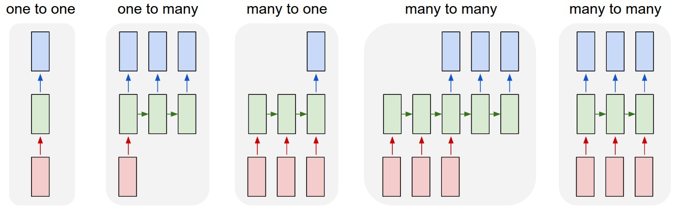
(1) One-to-One        (2) One-to-Many       (3) Many-to-One
    (vanilla network)     (image captioning)     (sentiment analysis)

     x                    x                  x₁ x₂ x₃ x₄
     ↓                    ↓                   ↓  ↓  ↓  ↓
   [NET]               [RNN]→[RNN]→[RNN]   [RNN]→[RNN]→[RNN]→[RNN]
     ↓                    ↓     ↓     ↓                       ↓
     y                   y₁    y₂    y₃                       y


(4) Many-to-Many      (5) Many-to-Many
    (synchronous, e.g. NER)  (asynchronous, e.g. translation)

 x₁ x₂ x₃ x₄         x₁ x₂ x₃    y₁ y₂ y₃ y₄
  ↓  ↓  ↓  ↓           ↓  ↓  ↓      ↓  ↓  ↓  ↓
[RNN]→[RNN]→[RNN]→[RNN] [Encoder]→c→[Decoder]
  ↓    ↓    ↓    ↓                    ↓  ↓  ↓  ↓
 y₁   y₂   y₃   y₄                  y₁ y₂ y₃ y₄
Type (5) is the Seq2Seq architecture (see the Seq2Seq notes for details).
Bidirectional RNN (BiRNN)
A unidirectional RNN can only see past information. However, many tasks require access to both preceding and following context:
- NER: "Apple Inc." — seeing "Inc." is needed to recognize "Apple" as an organization name
- Cloze test: "I ___ football" — requires seeing both sides
BiRNN uses two independent RNNs to process the sequence from left-to-right and from right-to-left, respectively:
Forward:  x₁ ──→ h⃗₁ ──→ h⃗₂ ──→ h⃗₃ ──→ h⃗₄
Backward: x₁ ←── h⃖₁ ←── h⃖₂ ←── h⃖₃ ←── h⃖₄

Final:    h₁ = [h⃗₁; h⃖₁]    h₂ = [h⃗₂; h⃖₂]    ...
          (concatenation of forward and backward hidden states)
The two directional RNNs have independent parameters and do not share weights. The final representation at each position contains complete contextual information.
Note: BiRNNs cannot be used for autoregressive generation (because when generating word \(t\), word \(t+1\) does not yet exist). They are mainly used for understanding tasks (classification, tagging, encoders, etc.).
Deep RNN (Stacked RNN)
Just like CNNs, RNNs can be stacked in multiple layers to increase depth:
Layer 3:  h₁⁽³⁾ ──→ h₂⁽³⁾ ──→ h₃⁽³⁾ ──→ y
           ↑           ↑           ↑
Layer 2:  h₁⁽²⁾ ──→ h₂⁽²⁾ ──→ h₃⁽²⁾
           ↑           ↑           ↑
Layer 1:  h₁⁽¹⁾ ──→ h₂⁽¹⁾ ──→ h₃⁽¹⁾
           ↑           ↑           ↑
          x₁          x₂          x₃
Each layer takes the hidden states from the layer below as its input. In practice, RNNs are typically stacked only 2-4 layers deep (unlike CNNs which can be stacked 100+ layers), because RNNs are already very "deep" along the temporal dimension, and adding depth in the layer dimension makes vanishing gradients even more severe.
Key Limitations of RNNs
| Limitation | Cause | Subsequent Solution |
|---|---|---|
| Vanishing gradient | Chain of products in BPTT → cannot learn long-range dependencies | LSTM / GRU (gating mechanisms) |
| No parallelism | \(h_t\) must wait for \(h_{t-1}\) | Transformer (Self-Attention) |
| Limited memory | Hidden state is a fixed-size vector; information loss increases with sequence length | Attention mechanism |
| Unidirectional information flow | Standard RNNs only see the past | BiRNN |
Can an RNN really remember the first chapter? No. Suppose the hidden state has \(d_h = 256\); then the information from an entire book (potentially hundreds of thousands of words) is compressed into 256 floating-point numbers. In theory, the information capacity is far from sufficient. Moreover, due to vanishing gradients, it is very difficult during training to make the model learn to retain early information. This is why LSTM (which uses gating for selective memory) and Attention (which directly accesses any historical position) are needed.
Comparative Summary with CNNs
| CNN | RNN | |
|---|---|---|
| Suitable data | Grid-structured (images) | Sequential (text, time series) |
| Core assumptions | Locality + spatial translation invariance | Temporal dependence + temporal translation invariance |
| Parameter sharing | Convolution kernels shared spatially | Weights shared across time steps |
| Information flow | Local → global (receptive field expands layer by layer) | Sequential (history accumulated step by step) |
| Maximum path length | \(O(\log n)\) (through stacking layers) | \(O(n)\) (must be transmitted step by step) |
| Parallelism | High (different positions in parallel) | Low (time steps are sequential) |
| Depth | Can be very deep (100+ layers, ResNet) | Typically shallow (2-4 layers) |
Next steps: → LSTM (solving vanishing gradients with gating mechanisms) → Seq2Seq (encoder-decoder architecture)