Probability and Statistics in Deep Learning

When I first studied probability theory and mathematical statistics, I always felt like I only half-understood them. So I decided to start a fresh set of notes, explaining these two concepts from first principles and re-examining what probability and statistics really are. These notes focus on content relevant to deep learning; unrelated material is omitted. For more detailed probability and statistics content, see the math notes.

Probability as a Tool

What is probability? Probability is an invented tool we use to compensate for our lack of omniscience. Probability is theoretical — it takes God's-eye view.

Probability theory encompasses two parts: probability and frequency. Probability defines the rules (random variables, expectations, distributions), while frequency establishes the connection between those rules and reality (the Law of Large Numbers, the Central Limit Theorem).

Modeling Ignorance

Everything must begin with ignorance. Clearly, if we could know every state of a system, then under classical mechanics — or rather, under our naive understanding of the world — flipping a coin would be a fully deterministic event.

Yet when anyone flips a coin, no one else can predict the outcome. This is fundamentally because we cannot observe all the variables and influencing factors throughout the entire coin-flipping process. We lack complete knowledge of the event, so we say coin-flipping is a chaotic system and our understanding is incomplete.

Clearly, we face several problems:

We cannot measure wind, gravity, angle, air resistance, and many other factors.
For any given factor, we cannot measure it precisely.
We also cannot write an equation that analytically solves such a complex system.

But we still want to know the result of a coin flip. So we begin attempting to model this chaotic system. Over the course of history, people ultimately discovered that "randomness" and "probability" are the most effective solutions to this problem — they are the most intuitive, simple enough for a schoolchild to use. In other words, probability is the most economical and effective tool we have for dealing with determinism too complex to compute.

After centuries of research on probability and randomness, two mainstream schools of thought have emerged:

Frequentist school: Probability is the limit of the relative frequency of an event over a large number of repeated trials. Even though each individual flip is deterministic, the macroscopic statistics still converge to 1/2.
Bayesian school: Probability is the degree of confidence under incomplete information. In other words, probability is not a property of the coin itself, but a measure of how much we know about the coin's state.

Random Variables

A Random Variable is the carrier of probability — it turns real-world events into numbers. Put another way, a random variable is a container that connects the real world to mathematical computation.

For example, "heads" is a physical phenomenon; mathematics cannot directly compute "heads + heads." So we need a "function" to map reality into numbers.

We define a variable \(X\):

If heads, we record \(1\).
If tails, we record \(0\).

This \(X\) is a random variable. Unlike an ordinary algebraic variable (such as \(x=5\)), where \(x=5\) is fixed, \(X\) is an unknown box — before you open it, you don't know whether it's 0 or 1, but you know the probability of it being 1 is 50%.

Expectation

The Expected Value (Expectation, \(E[X]\) or \(\mu\)) is the theoretical average computed from probabilities. Expectation is about probability.

For example, suppose you play a dice game:

Roll 1–5: you lose 1 yuan.
Roll 6: you win 5 yuan.

This defines a random variable \(X\):

\[ E[X] = (-1 \times \frac{5}{6}) + (5 \times \frac{1}{6}) = 0 \]

The expectation is a fixed value.

Distribution

The expected value gives us one number: the theoretical average. But can we derive the overall picture of all possible outcomes based on their probabilities?

A Distribution is the complete inventory of probabilities — it shows what the possibilities of all outcomes look like. In other words, we plot the results according to their probabilities, and what we get is the distribution. Therefore, a distribution is also an idealized concept — a God's-eye concept.

Model Parameters

When God creates a distribution, it's not drawn arbitrarily — it's determined by adjusting a few key knobs. These knobs are the parameters.

For coin-flipping, God's knob is called P — the probability of heads. If P is set to 0.5, the coin is fair; if P is set to 0.8, the coin is biased. This P is the model parameter.

For the distribution of heights, God has two knobs: the mean and the variance. The mean determines where the peak is — for instance, the average height is 170 cm. The variance determines how wide the peak is — whether everyone's height is roughly the same, or widely spread out.

Model parameters are the core settings that determine the stochastic laws of the world.

Common distributions include:

Bernoulli distribution — the coin-flip distribution, with only one parameter P (probability of heads).
Poisson distribution — like waiting for a bus, with only one parameter λ (average rate of occurrence).
Exponential distribution — for lifetimes, with only one parameter λ (decay rate).

Frequency and Limit Theorems

If probability is the script, then frequency is the performance. Probability is fixed; frequency is not. Probability belongs to God; frequency belongs to mortals.

Obviously, studying the case where frequency = 1 (i.e., flipping a coin once) is not very meaningful. We want to discover patterns, so from the frequency perspective, we primarily study the deterministic regularities that random phenomena exhibit as the number of trials approaches infinity.

Independent and Identically Distributed Samples

Independent and Identically Distributed Samples (I.I.D. Samples).

Now you actually start playing the game:

First roll: you get 3, lose 1 yuan (\(x_1 = -1\)).
Second roll: you get 6, win 5 yuan (\(x_2 = 5\)).
Third roll: you get 2, lose 1 yuan (\(x_3 = -1\)).

These specific numbers \(-1, 5, -1\) are the samples.

Frequency

Frequency is the proportion of times a particular outcome occurs relative to the total number of trials in your experiment.

For example, you start flipping coins. You flip 10 times and get heads 8 times — the frequency of heads is 0.8. You flip 100 times and get heads 60 times — the frequency of heads is 0.6.

Frequency is the value we record from our experiments.

Empirical Distribution

When we refer to a "distribution," we usually mean the probability distribution, not the frequency distribution. To avoid confusion, in practice I recommend using the term Empirical Distribution to refer to the frequency distribution.

An empirical distribution is what you get when you plot all of your experimental results, typically using a histogram.

Sample Mean

The Sample Mean (\(\bar{X}\)) is simply the sum of your experimental results divided by the number of trials.

It is essential to remember: the sample mean is a random variable. The expected value does not change, but the sample mean does. You play a few rounds of the game and get a sample mean, then play a few more, and the sample mean may shift. In other words, the sample mean always fluctuates with luck.

Law of Large Numbers

The Law of Large Numbers (LLN) is the destiny of frequency — it states that given enough trials, luck becomes certainty.

The Law of Large Numbers is truly remarkable:

As long as the number of trials (\(n\)) is large enough, the sample mean (\(\bar{X}\)) will inevitably converge to the God's-eye expected value (\(\mu\)).

Distribution?

Tiny random factors?

Central Limit Theorem

The Central Limit Theorem is abbreviated CLT. Here, "Central" means "most important" or "most fundamental" — it conveys that this theorem is the most central and important result in the discipline. "Limit" refers to the mathematical limit: as the sample size approaches infinity, the distribution of the sample mean converges to a normal distribution.

A one-sentence summary of its literal meaning:

The most central theorem in probability theory states that as the sample size approaches infinity, the distribution converges to the normal distribution.

Put differently, if probability is God's script, then the CLT tells us: even the errors in the script follow a pattern. The concept of likelihood, which we will learn later, is our tool for guessing the script.

The Central Limit Theorem (CLT) is the advanced version of the Law of Large Numbers. The LLN tells us that after flipping a coin infinitely many times, the average proportion of heads will converge to 50%. But what does the overall distribution of all the coin outcomes look like?

The magic of the CLT is this: no matter what the original distribution of the random variable is (even if it's a jagged shape, a coin with only 0 and 1, or a die), as long as you add up (or average) many independent random variables, the distribution of these sums will eventually become a normal distribution (bell curve). This explains why normal distributions are so common in nature (height, measurement errors, noise) — they are all the result of countless tiny random factors being superimposed. As long as the quantity is large enough, the error distribution will be normal.

In the real world, data always contains errors. We call these errors Noise. The sources of these errors are varied and impossible to fully identify. However, we can reasonably assume: the factors causing these errors consist of countless tiny, mutually independent influences.

Since errors are caused by the superposition of countless tiny factors, then by the Central Limit Theorem, the distribution of the total error must be a normal distribution! This is precisely why, when designing loss functions, we can boldly assume: the error between predicted and true values follows a normal distribution.

If we don't trust the CLT, we can no longer use MSE. Why? Because:

Our data inherently contains errors, and these errors are the superposition of countless tiny factors.
Since errors are the superposition of countless independent tiny factors, the distribution of the total error must be a normal distribution (Central Limit Theorem).
Since errors follow a normal distribution, we can write out the probability density function. The PDF is: \(P(\epsilon) = \frac{1}{\sqrt{2\pi}\sigma} e^{-\frac{\epsilon^2}{2\sigma^2}}\).
We know that error = true value - predicted value. In other words, \(\epsilon = y - \hat{y}\). Substituting this into the probability density function above, we get the error's probability density: \(P(y | \hat{y}) = \frac{1}{\sqrt{2\pi}\sigma} e^{-\frac{(y - \hat{y})^2}{2\sigma^2}}\). This formula computes: given that the prediction is \(\hat{y}\), what is the likelihood that the true value y occurs.
Now that we know the probability for one prediction, we can obtain the likelihood for N predictions. Likelihood = the product of all sample probabilities. Suppose we want to predict N house prices: \(L = \prod_{i=1}^N P(y_i | \hat{y}_i) = \prod_{i=1}^N \left( \frac{1}{\sqrt{2\pi}\sigma} e^{-\frac{(y_i - \hat{y}_i)^2}{2\sigma^2}} \right)\)
We want to find the maximum of the likelihood function, but multiplying probabilities together is computationally difficult. So we take the logarithm of everything, converting multiplication into addition — this gives us the log-likelihood. After the conversion, we drop the constant terms, since constants do not affect the location of the maximum. Thus, we are left with finding the maximum of: \(\sum_{i=1}^N -\frac{(y_i - \hat{y}_i)^2}{2\sigma^2}\)
Applying the mathematical transformation to negative log-likelihood, this becomes finding the minimum. We also drop the constant in the denominator, which does not affect the location of the extremum: \(\text{Minimize } \sum_{i=1}^N (y_i - \hat{y}_i)^2\). This is SSE (Sum of Squared Errors). Dividing by the sample size N gives MSE (Mean Squared Error).

Statistics

Probability theory works in the forward direction — given the parameters, we deduce the resulting data from God's perspective. Statistics, on the other hand, works in reverse.

For example, if we pick up a coin and don't know whether it's fair, we run an experiment — flip it 10 times — and try to infer whether the coin is fair.

If probability and parameters are set by God, then statistics is the process of using mortal data to crack the parameters God has set.

Statistical Inference and Parameter Estimation

Statistical inference is a very broad field within statistics. In general, it is about using sample data to infer characteristics of the population. Statistical inference encompasses parameter estimation, hypothesis testing, prediction, and more. In deep learning, parameter estimation is by far the most commonly used.

Parameter estimation is a specific type of task within statistical inference. Its goal is clear: compute the value of the unknown number (parameter) in the model. It does not care whether the number is correct (that's what hypothesis testing is for) — it only cares what the number is.

Likelihood

Likelihood is the "plausibility" that a parameter takes a certain value, given that the data has already been observed.

For example, suppose we set the probability of heads at 0.5, then flip the coin once and observe heads. This is now an ironclad fact — it cannot be changed.

Now, we have two suspect coins to choose from:

A coin with P=0.1 (only 10% chance of heads) — call it Coin 1.
A coin with P=0.9 (90% chance of heads) — call it Coin 2.

Coin 1 has only a 0.1 probability of producing heads, yet it happened on our watch — that would be practically a miracle. Since it would be a miracle, we consider it highly unlikely that Coin 1 is the culprit. We say Coin 1 has low likelihood.

Conversely, Coin 2 has a 90% probability of producing heads, so the coin in our hand is much more likely to be Coin 2. We say Coin 2 has high likelihood.

In other words, when an event has already occurred, whichever explanation makes that event more probable has higher likelihood.

The likelihood value we refer to here is the specific numerical value of the likelihood. For Coin 1, when P=0.1, the likelihood value = 0.1; for Coin 2, when P=0.9, the likelihood value = 0.9.

In other words, the likelihood of a single sample is simply that sample's probability under the assumed probability model.

\[ \underbrace{L(\theta | x)}_{\text{似然度}} = \underbrace{P(x | \theta)}_{\text{在理想分布下的概率值}} \]

The parameter defines the ideal probability distribution curve, the sample data is the real-world data point, and the likelihood is the height on the ideal curve corresponding to that real-world data point.

Likelihood Function

The Likelihood Function is a formula — or equivalently a curve — that contains all possible values of P (from 0 to 1) along with their corresponding plausibilities.

Let's look at the coin-flipping example.

Suppose we flip a coin 10 times and get heads 7 times. The question is: Is this coin fair?

From a probability perspective, if we assume the coin is fair, then the probability is 0.5, denoted \(\theta = 0.5\).

We can then compute the likelihood of the 10-flip outcome. The likelihood is the product of each flip's probability. For 10 flips with 7 heads and 3 tails, under the assumed probability of 0.5, the likelihood is:

\[ L(\theta = 0.5) = \theta^7 \times (1-\theta)^3 = 0.00097 \]

Note that the likelihood above is for one specific ordering (e.g., HHHHHHHTT T). In reality, we must also account for the different arrangements:

\[ \binom{10}{7} = \frac{10 \times 9 \times 8}{3 \times 2 \times 1} = 120 \]

Therefore, the final likelihood of 7 heads and 3 tails = 0.00097 * 120 = 0.117.

Similarly, we can compute the likelihood for \(\theta\) = 0.7, which turns out to be 0.2668.

If we find the likelihood values for all \(\theta\), they naturally form a curve. Plotting this curve — that is, plotting the likelihood function for coin-flipping — gives us the following figure:

1770758773807

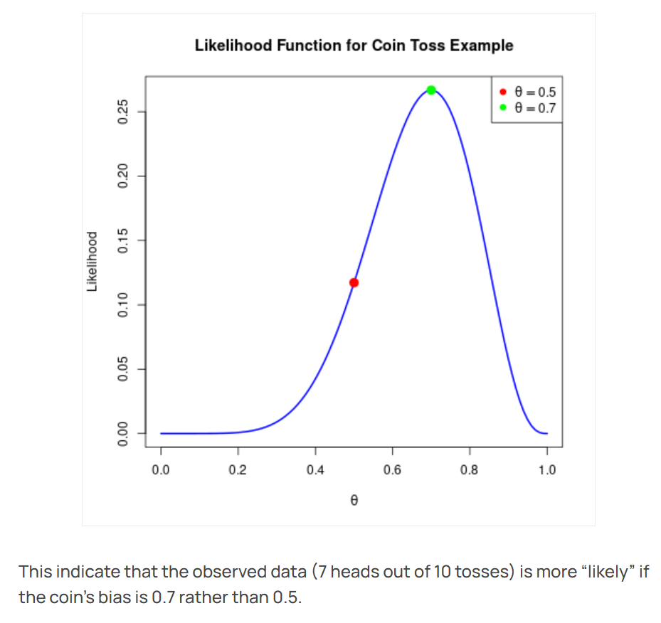
The X-axis represents the parameter P we are trying to guess. If P = 0.5, the coin is fair.

The Y-axis represents the likelihood. The blue line is the likelihood function. We can see that if we assume the coin is fair, the likelihood is low; if we assume the coin is biased, the likelihood is high.

In this case, the green dot at \(\theta = 0.7\) is the maximum likelihood estimate. In other words, having flipped the coin 10 times and observed 7 heads, if we estimate using maximum likelihood, our best guess is that the coin's true parameter is most likely P = 0.7.

Suppose you collect a set of data \(x_1, x_2, ..., x_n\) (e.g., the heights of all students in a class).

The normal distribution formula (probability density function, PDF) looks like this:

\[ f(x) = \frac{1}{\sqrt{2\pi}\sigma} e^{-\frac{(x-\mu)^2}{2\sigma^2}} \]

The likelihood function \(L(\mu, \sigma)\) is the product of each data point's probability:

\[ L(\mu, \sigma) = P(x_1) \times P(x_2) \times ... \times P(x_n) \]

The expanded formula is quite long, but you only need to know its inputs and outputs:

Input: two variables \(\mu\) (mean) and \(\sigma\) (standard deviation).
Output: a numerical value \(L\) (the likelihood — i.e., "how well this set of parameters explains the current data").

Because there are two input variables (\(\mu\) and \(\sigma\)), the likelihood function is no longer a curve on a plane but rather a surface in three-dimensional space.

X-axis: represents \(\mu\) (the guessed mean, e.g., 160, 170, 180...)
Y-axis: represents \(\sigma\) (the guessed spread, e.g., 5, 10, 20...)
Z-axis (height): represents the likelihood.

Its shape resembles a mountain (or a mound).

The base of the mountain: represents absurd parameter combinations (e.g., guessing the class average height is 100 cm with a spread of 0.1 cm) — likelihood near 0.
The slopes: represent parameters that are starting to become reasonable — likelihood rises.
The peak (summit): represents the most perfect parameter combination.

Maximum Likelihood Estimation

Maximum Likelihood Estimation (MLE) is a method for accomplishing the task of parameter estimation. Its logic is: "Find the parameter that, if used to generate data, would make the probability of the currently observed data the greatest."

When we know nothing about the world and can only see the outcome, accepting the parameter that makes that outcome most probable is the most rational choice.

A detective analogy: You walk into a room and find a puddle of water on the floor (the data). Now there are two suspect explanations (parameters):

Explanation A: Someone just spilled a glass of water (probability of a spill causing a wet floor = 99%).
Explanation B: The roof leaked, but today is a sunny day (probability of a leak on a sunny day causing a wet floor = 0.001%).

As a detective (statistician), which would you choose? You'd choose A. Why? Because Explanation A makes "water on the floor" seem most plausible.

This is the meaning of MLE: In the coin-flipping example, \(\theta=0.7\) maximizes the probability of "7 heads out of 10 flips." If you insist that \(\theta=0.1\) (only 10% chance of heads), you're forcing an explanation of a near-miracle — that's not scientific.

In other words, MLE is saying: the statistical result represents the most likely parameter. Its subtext is: data doesn't lie. If the data looks like this, then the underlying parameter is most probably like that.

Although this may sound like stating the obvious, in mathematics and practice, it is the optimization process itself.

An important caveat: we must use MLE in conjunction with the Law of Large Numbers. For example, if you flip a coin just once and get heads, MLE would estimate P = 1, meaning the coin always lands heads — clearly unreasonable. Therefore, we must increase the sample size, making it large enough so that by the Law of Large Numbers, the sample mean converges to the expected value, and the MLE estimate converges to the truth.

Let's use the example from the Likelihood Function section above to illustrate:

We observe data (frequencies).
We assume these data follow some distribution (e.g., a coin-flip distribution).
But we don't know the parameter of this distribution (what is \(P\)?).
So we write out a likelihood function.
We want to find a \(P\) that maximizes the likelihood function.
This is statistical inference.

In plain language:

"Since the event has already happened (the data), I'll accept that the parameter God set must be the one that makes this event most probable."

Let's look at MLE using the normal distribution example from the Likelihood Function section. In the coin example, we were finding the highest point on a curve. In the normal distribution example, we are finding the highest peak (summit) on a mountain.

When you stand at the summit, the coordinates beneath your feet \((\mu, \sigma)\) are the answer we seek:

This is the mean that best fits the current data.
This is the variance that best fits the current data.

Let's see why MLE comes up in AI training. We know that the essence of training a deep neural network is finding the true parameters. We can therefore say: the essence of training AI is getting it to guess the correct answer.

Modern AI models have hundreds of billions of parameters. Their likelihood function is an astronomically complex landscape in hundreds of billions of dimensions. Training AI means finding the highest peak.

Suppose the neural network's parameters are W. We want to maximize the likelihood:

\[ \text{maximize } L(W) = \prod P(\text{true label} | \text{input}, W) \]

Here, P is computed by the neural network — for example, the softmax output — and P is determined by W.

Note that in AI training, we are indeed performing Maximum Likelihood Estimation (MLE), trying to find a set of parameters that maximizes the probability of the data. However, directly computing the "likelihood function" poses two enormous difficulties:

Numerical underflow. Likelihood involves multiplying many probabilities together, so as the sample size grows, the value approaches 0, and the computer will simply record it as 0.
Products are hard to differentiate.

So in practice, we perform two operations:

Take the logarithm. The logarithm converts multiplication into addition, turning the product into a sum. Moreover, the logarithm is monotonically increasing, so the maximum of the original function remains the maximum after the transformation. At this point, we call it the Log-Likelihood, and we are still looking for the highest point.
Negate. In optimization, we conventionally think of the objective as an error or loss, so we want it to be as small as possible. Therefore, we add a negative sign, yielding the Negative Log-Likelihood (NLL).

After these operations, maximizing the likelihood becomes minimizing the negative log-likelihood. The highest peak of the likelihood function becomes the lowest valley of the negative log-likelihood function. This is the difference between the statistical perspective of maximizing likelihood (climbing the mountain) and the engineering perspective of minimizing loss (descending the mountain).

Among commonly used AI loss functions, cross-entropy loss is precisely the negative log-likelihood.

Now, let's return to neural networks. Using a CNN that classifies images as cats or dogs as an example:

Input (\(x\)): an image.
Parameters (\(W\)): the hundreds of millions of weights in the CNN (initially random numbers).
Output (\(P\)): the probabilities output by the softmax layer.

In the first round of training, the results are as follows:

Image 1 (true: cat): the CNN guesses randomly, outputting \(P(\text{cat}) = 0.1\).
Image 2 (true: dog): the CNN guesses randomly, outputting \(P(\text{dog}) = 0.2\).
Image 3 (true: cat): the CNN guesses randomly, outputting \(P(\text{cat}) = 0.3\).

The likelihood at this point is the probability of correctly guessing the true labels of these three images under the current set of parameters W.

Note that when computing the likelihood, we only consider the probability assigned to the true class. For example, Image 1's CNN output certainly includes probabilities for other classes, since the softmax outputs must sum to 1. But for these three images, we only consider the probability values assigned to the true labels.

Clearly, the current likelihood is:

\[ L = 0.1 \times 0.2 \times 0.3 = \mathbf{0.006} \]

This \(0.006\) is very low! In the ideal case, if all three images were classified correctly with full confidence, the likelihood would be:

\[ L_{ideal} = 1.0 \times 1.0 \times 1.0 = \mathbf{1.0} \]

But the current likelihood is 0.006, far below the ideal. This indicates that the current parameters \(W\) are extremely unreliable. Although we don't know the actual maximum of the likelihood function, nor whether the ideal L = 1.0 is truly attainable, we know the gap between the current L and the ideal L is enormous — so we need to train the model.

Imagine we have the likelihood function over the parameters W, and our goal is to find its highest point. We are clearly not there yet. To maximize the likelihood L, we use the mathematical trick mentioned above: convert "maximize likelihood" into "minimize the negative log-likelihood," then use backpropagation and optimization techniques to update the parameters, gradually training toward the maximum likelihood result.

Information Theory

Maximum Entropy

This is a principle for choosing a probability model when information is insufficient.

Core idea: Among all possible probability distributions that satisfy the known constraints (e.g., the mean must equal a certain value), we should choose the one that is most "uncertain" (i.e., has the greatest entropy).

In many cases (especially for exponential family distributions, such as the Gaussian distribution, Poisson distribution, etc.), the maximum entropy principle and maximum likelihood estimation are equivalent.