LR Scheduling

Learning Rate Scheduling

Another major challenge in DNN training is setting an appropriate learning rate schedule. A poor choice can lead to:

• Training instability
• Slow convergence
• Convergence to suboptimal solutions

Learning Rate Schedulers play a crucial role in deep learning training. By dynamically adjusting the learning rate, they help the model learn rapidly in the early stages and optimize steadily and precisely in later stages, thereby improving both convergence speed and final model performance.

More specifically, the learning rate is the step size that optimizers (such as SGD or Adam) use when updating model parameters. If the step is too large, the optimizer may overshoot the optimum; if it is too small, convergence will be excessively slow. Schedulers are mechanisms that automatically manage and adjust this step size. Rather than using a fixed learning rate, they modify it according to predefined rules (e.g., based on the epoch number or changes in the loss value).

Their specific roles are as follows:

• Fast Progress Early On: At the beginning of training, model parameters are far from their optimal values, so a large learning rate can be used. This allows the model to traverse flat regions of the loss landscape quickly, find the general "direction" of the loss function, and achieve rapid convergence.
• Stable Fine-Tuning Later: As training progresses, parameters approach the minimum of the loss function. Continuing with a large step size would cause the model to oscillate around the optimum without converging stably. The scheduler therefore reduces the learning rate, allowing the model to take smaller steps for stable, precise optimization (fine-tuning), ensuring a more accurate minimum is found.

Ultimately, large steps in the early phase allow the model to reach an acceptable performance level more quickly, while tiny steps in the later phase enable it to locate the global (or local) minimum of the loss function more precisely, yielding higher accuracy and lower loss.

A learning rate scheduler is like the accelerator and brake of a car. When starting out (early training), you press the accelerator hard (high learning rate) to gain speed quickly; as you approach the destination (late training), you gently apply the brake (low learning rate) to stop slowly and precisely. This dynamic control is a key technique for improving efficiency and accuracy in deep learning.

---

Line Search and the Optimization Perspective on Learning Rates

In classical optimization theory, each gradient descent (GD) update involves choosing an appropriate step size \(\lambda_k\):

\[ \theta^{(k+1)} = \theta^{(k)} - \lambda_k \cdot \nabla J(\theta^{(k)}) \]

Note that in the original gradient descent method (from the optimization field, not machine learning), the step size \(\lambda_k\) may differ at each iteration \(k\). It is typically determined via line search -- searching along the update direction \(\Delta\theta^{(k)}\) for a step size that sufficiently decreases the loss function.

Backtracking Line Search: Starts with a large step size and gradually reduces it until a sufficient decrease condition (Armijo condition) is satisfied.

Exact Line Search: Exactly solves the one-dimensional optimization problem \(\min_{\lambda > 0} J(\theta^{(k)} - \lambda \nabla J(\theta^{(k)}))\).

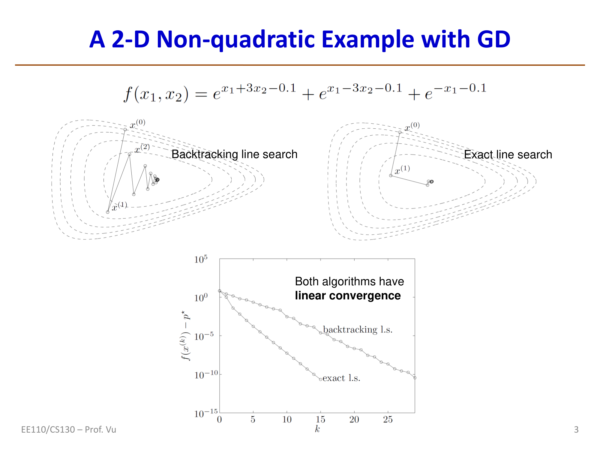
The figure above illustrates the optimization of the function \(f(x_1, x_2) = e^{x_1+3x_2-0.1} + e^{x_1-3x_2-0.1} + e^{-x_1-0.1}\). The backtracking line search trajectory exhibits a zigzag pattern, while the exact line search path is more direct. Both algorithms exhibit linear convergence.

However, performing a line search at every step is computationally prohibitive in DNN training. Researchers have therefore focused on designing learning rate schedules or rules that automatically update the learning rate without numerical search.

---

Sufficient Conditions for SGD Convergence (Robbins-Monro Conditions)

For the SGD update \(\theta^{k+1} \leftarrow \theta^k - \lambda_k \cdot g(\theta^k)\), where \(g(\theta^k)\) is a stochastic estimate of the gradient, convergence requires the following sufficient conditions:

\[ \sum_{k=1}^{\infty} \lambda_k = \infty \quad \text{and} \quad \sum_{k=1}^{\infty} \lambda_k^2 < \infty \tag{C} \]

Intuition:

• The first condition \(\sum \lambda_k = \infty\) ensures that the cumulative step sizes are large enough for the optimization process to reach any point in the parameter space.
• The second condition \(\sum \lambda_k^2 < \infty\) ensures that the step sizes eventually become small enough for the influence of noise to vanish, allowing convergence to a stable solution.

Important note: Condition (C) is a sufficient but not necessary condition -- satisfying (C) guarantees SGD convergence, but SGD can converge without (C). Since the second condition requires a decreasing learning rate, this provides the theoretical foundation for decaying learning rate schedulers.

In practice, many learning rate schedulers satisfy these conditions: starting from a maximum value \(\lambda_{max}\), gradually decaying to a minimum value \(\lambda_{min}\), and remaining there. Different schedulers differ in their choice of the decay function \(f(k, \lambda_0)\). Since actual training stops after a finite number of steps \(k\), such decreasing schedules generally work well.

---

Step Decay

Step Decay is the simplest and most classic learning rate scheduling strategy. The core idea is to multiply the learning rate by a decay factor (typically 0.1 or 0.5) every fixed number of epochs.

Formula:

\[ \eta_t = \eta_0 \cdot \gamma^{\lfloor t / S \rfloor} \]

where \(\eta_0\) is the initial learning rate, \(\gamma\) is the decay factor (e.g., 0.1), \(S\) is the step size (how many epochs between each decay), and \(\lfloor \cdot \rfloor\) is the floor operation.

Typical setup: In the classic ImageNet ResNet training configuration, the initial learning rate is \(\eta_0 = 0.1\), and the learning rate is multiplied by 0.1 every 30 epochs (i.e., decayed at epochs 30, 60, and 90).

Advantages: Simple to implement, produces stable results, and is the default choice in many classic papers.

Disadvantages: Requires manual selection of the decay timing and magnitude, lacking flexibility; the abrupt change in learning rate can cause brief instability in the training loss.

The corresponding PyTorch implementations are torch.optim.lr_scheduler.StepLR and MultiStepLR.

---

Exponential Decay

Exponential Decay smoothly reduces the learning rate according to an exponential function, avoiding the sudden jumps that occur with Step Decay.

Formula:

\[ \eta_t = \eta_0 \cdot \gamma^{t} \]

where \(\gamma \in (0, 1)\) is the per-epoch decay rate, e.g., \(\gamma = 0.95\) or \(\gamma = 0.99\).

Characteristics: The learning rate follows a smooth exponential curve, decreasing rapidly at first and more slowly later. Compared to Step Decay, exponential decay is smoother and avoids sudden learning rate jumps. However, careful selection of \(\gamma\) is important: if \(\gamma\) is too small, the learning rate decays too quickly, potentially leading to insufficient training; if \(\gamma\) is too close to 1, the decay is too slow and barely differs from a constant learning rate.

The corresponding PyTorch implementation is torch.optim.lr_scheduler.ExponentialLR.

---

Inverse Square Root Decay

Inverse Square Root Decay is a classic schedule that satisfies the Robbins-Monro conditions and is widely used in the Transformer's Noam scheduler:

\[ \lambda_t = \frac{\lambda_0}{\sqrt{t}} \]

This is a special case of polynomial decay \(\lambda_k = \lambda_0 / (k+1)^p\) with \(p = 0.5\). The decay rate is moderate -- slower than exponential decay but faster than linear decay -- making it particularly suitable for scenarios requiring long training.

---

Convergence Analysis

Several important conclusions can be drawn regarding the convergence properties of different schedulers:

Effect of the decay path: The specific shape of the learning rate decay function is not the most critical factor. Most convergence analyses use the polynomial learning rate \(\lambda_t = \lambda_0 / \sqrt{t}\) as the subject of analysis. Different variants may affect the stability of the loss curve, but should not affect whether the algorithm converges.

Convergence steps for polynomial learning rates: For the polynomial learning rate \(\lambda_k = \lambda_0 / (k+1)^p\) (\(p \in (0,1)\)), the number of steps required to achieve an optimality gap \(\|J(\theta^k) - J(\theta^*)\|\) below a certain threshold is:

\[ N^* = m^{\frac{1}{(1-p)c}} \]

where \(m\) is the number of data samples, \(p\) is the polynomial exponent, and \(c\) is a constant. (See Yao 2007, Early Stopping)

Intuition:

• Larger datasets (larger \(m\)) lead to longer training times
• Smaller \(p\) (\(0 < p < 1\)) yields a smaller \(N^*\), meaning more aggressive learning rate decay leads to shorter training times. This explains why exponential decay converges faster in certain scenarios.

---

Cosine Annealing

Cosine Annealing is a highly popular learning rate scheduling strategy, proposed by Loshchilov and Hutter in their 2016 SGDR (SGD with Warm Restarts) paper.

Formula:

\[ \eta_t = \eta_{min} + \frac{1}{2}(\eta_{max} - \eta_{min})\left(1 + \cos\left(\frac{t}{T}\pi\right)\right) \]

where \(\eta_{max}\) is the maximum learning rate (usually equal to the initial learning rate), \(\eta_{min}\) is the minimum learning rate (usually 0 or a very small value), \(T\) is the total number of training periods, and \(t\) is the current period.

Why it works:

• Early in training, the high learning rate enables rapid exploration of the parameter space
• In the middle of training, the learning rate decreases gradually for progressive refinement
• Late in training, the learning rate approaches zero for fine-grained search near local optima
• The shape of the cosine curve causes the learning rate to change slowly at the beginning and end but more rapidly in the middle, which better suits actual training needs than linear decay

Warm Restarts (SGDR): The core idea of SGDR is to periodically "restart" the learning rate back to its initial value, then decay it again following a cosine curve. The benefit of this strategy is that when the learning rate suddenly increases, the model can escape its current local optimum and explore potentially better solutions. Each subsequent cosine decay then allows the model to converge stably. In practice, the restart period can be progressively lengthened (e.g., \(T_0, 2T_0, 4T_0, \ldots\)), allowing more exploration early on and more convergence later.

The corresponding PyTorch implementations are torch.optim.lr_scheduler.CosineAnnealingLR and CosineAnnealingWarmRestarts.

---

Warmup

Warmup (learning rate warmup) refers to linearly increasing the learning rate from a very small value (such as 0 or \(10^{-7}\)) to the target learning rate over the first few training steps, before applying another strategy (such as cosine annealing) for decay.

Linear Warmup formula:

\[ \eta_t = \eta_{target} \cdot \frac{t}{T_{warmup}}, \quad t \leq T_{warmup} \]

where \(T_{warmup}\) is the number of warmup steps and \(\eta_{target}\) is the target learning rate.

Why Warmup is needed:

1. Parameter instability early in training: Model parameters are randomly initialized, so the direction and magnitude of initial gradients are unreliable. Starting with a very large learning rate may push the model into poor regions of the parameter space or even cause divergence.
2. Inaccurate statistics in adaptive optimizers: For adaptive optimizers like Adam, the first- and second-moment estimates are highly inaccurate at the start of training (due to too few samples), and a large learning rate would cause abnormally large parameter updates.
3. Necessity for large-batch training: When using very large batch sizes (thousands or even tens of thousands), gradient estimates are very accurate (low variance). Directly using a large learning rate can cause the model to converge prematurely to sharp local minima with poor generalization. Warmup provides a buffer period for the parameters to "warm up" within a reasonable range.
4. Standard practice for Transformer training: The Noam scheduler used in the original Transformer paper (Vaswani et al., 2017) includes a warmup phase. Its learning rate formula is:

\[ \eta_t = d_{model}^{-0.5} \cdot \min(t^{-0.5}, \; t \cdot T_{warmup}^{-1.5}) \]

The learning rate increases linearly for the first \(T_{warmup}\) steps and then decays as \(t^{-0.5}\). Virtually all modern Transformer models (BERT, GPT, ViT, etc.) use warmup.

Theoretical motivation for Warmup: From the Hessian perspective, early in training, parameters are far from the optimum and the curvature of the loss surface (Hessian eigenvalues) can be very large and unstable. The optimal learning rate \(\lambda \approx 1/h\) (where \(h\) is a Hessian diagonal element) is therefore small. Directly using a large learning rate would produce an update \(\lambda \cdot g\) far exceeding the Newton step size, causing parameters to jump to worse regions or even diverge. Warmup allows the learning rate to gradually increase from a small value, giving the model time to stabilize gradient statistics and Hessian estimates.

---

OneCycleLR

OneCycleLR (1Cycle Policy), proposed by Leslie Smith in 2018, is based on the key finding that using a much larger learning rate than traditional methods, combined with a special scheduling strategy, can achieve Super-Convergence -- reaching better results with fewer training steps.

Strategy description:

The entire training process is divided into two phases:

1. Ascending phase (approximately the first 30%-45% of training): The learning rate linearly increases from a low value to the maximum learning rate \(\eta_{max}\)
2. Descending phase (approximately the last 55%-70% of training): The learning rate decays from the maximum value via cosine annealing to a very small value (approaching 0)

Simultaneously, the momentum varies inversely: momentum decreases when the learning rate rises and increases when the learning rate falls.

Super-Convergence: Smith found that with the 1Cycle Policy, the maximum learning rate can be set 3-10 times higher than in traditional methods. Combined with this "rise-then-fall" strategy, the model can achieve equivalent or even better performance using only 1/5 to 1/10 of the training steps required by traditional methods. This phenomenon is called super-convergence.

How to choose the maximum learning rate: Use the LR Range Test: gradually increase the learning rate from a very small to a very large value, recording the loss at each learning rate. Select the learning rate at the point where the loss decreases most rapidly as \(\eta_{max}\).

The corresponding PyTorch implementation is torch.optim.lr_scheduler.OneCycleLR.

---

ReduceLROnPlateau

ReduceLROnPlateau (plateau-based learning rate reduction) is an adaptive scheduling strategy. Rather than relying on a predefined decay schedule, it monitors a metric (typically validation loss) and automatically reduces the learning rate when the metric fails to improve for several consecutive epochs.

Mechanism:

• The monitored metric (e.g., validation loss) has not improved for patience epochs
• The learning rate is multiplied by factor (typically 0.1 or 0.5)
• A min_lr can be set to prevent the learning rate from dropping too low
• A threshold can be set to define the minimum magnitude of "improvement"

Typical setup: patience=10, factor=0.1 -- if the validation loss does not decrease for 10 consecutive epochs, the learning rate is reduced to 1/10 of its current value.

Advantages: No need to know the optimal decay timing in advance; the schedule is entirely driven by training performance. Particularly suitable for scenarios where the required number of training epochs is uncertain.

Disadvantages: It is a reactive strategy that only reduces the learning rate after detecting performance stagnation, introducing a certain degree of lag.

The corresponding PyTorch implementation is torch.optim.lr_scheduler.ReduceLROnPlateau.

---

Scheduler Comparison Summary

Scheduling Strategy	Core Mechanism	Hyperparameters	Typical Use Cases
Step Decay	Multiply by decay factor every fixed number of epochs	Step size, decay factor	CNN classification (ResNet, etc.)
Exponential Decay	Multiply by fixed decay rate each epoch	Decay rate \(\gamma\)	General purpose, when smooth decay is desired
Cosine Annealing	Follow a cosine curve from high to low	Max/min learning rate, period \(T\)	Mainstream choice for modern training
Warmup	Linearly increase learning rate at start of training	Number of warmup steps	Transformers, large-batch training
OneCycleLR	Rise then fall + inverse momentum variation	Max learning rate, total training steps	Fast convergence, super-convergence
ReduceLROnPlateau	Reduce learning rate when monitored metric stagnates	patience, factor	Scenarios with uncertain training duration

Practical recommendations:

• For training Transformer-based models, the combination of Warmup + Cosine Annealing is recommended
• For training CNN classification models, both Step Decay and Cosine Annealing are good choices
• For fast training, consider OneCycleLR
• When the task is not well understood or the appropriate number of epochs is unclear, ReduceLROnPlateau serves as a reliable fallback
• In virtually all large-scale training scenarios, Warmup is indispensable

---

Polynomial Decay

Polynomial Decay reduces the learning rate from the initial value to the minimum value following a polynomial function:

\[ \eta_t = (\eta_0 - \eta_{min}) \cdot \left(1 - \frac{t}{T}\right)^p + \eta_{min} \]

where \(p\) is the polynomial exponent. When \(p = 1\), this becomes Linear Decay, where the learning rate decreases uniformly from \(\eta_0\) to \(\eta_{min}\).

Linear Decay is the default choice for training BERT and many NLP models. A typical configuration is Warmup + Linear Decay: linearly increase the learning rate for the first few steps, then linearly decay it to 0.

# PyTorch - Warmup + Linear Decay
from transformers import get_linear_schedule_with_warmup

scheduler = get_linear_schedule_with_warmup(
    optimizer,
    num_warmup_steps=1000,
    num_training_steps=total_steps
)

The corresponding PyTorch implementation is torch.optim.lr_scheduler.PolynomialLR.

---

Combining Schedulers

In practice, schedulers are often used in combination. The most common combination is Warmup + main scheduler:

import torch.optim as optim
from torch.optim.lr_scheduler import SequentialLR, LinearLR, CosineAnnealingLR

optimizer = optim.AdamW(model.parameters(), lr=1e-3, weight_decay=0.01)

# Warmup: linearly increase from 0.01*lr to lr over the first 1000 steps
warmup = LinearLR(optimizer, start_factor=0.01, total_iters=1000)

# Main scheduler: Cosine Annealing
cosine = CosineAnnealingLR(optimizer, T_max=total_epochs - 1000)

# Combine: Warmup first, then Cosine
scheduler = SequentialLR(optimizer, [warmup, cosine], milestones=[1000])

Common combinations:

Combination	Use Case
Warmup + Cosine Annealing	Transformer pretraining, ViT
Warmup + Linear Decay	BERT/GPT fine-tuning
Warmup + Cosine with Warm Restarts	Long training runs requiring strong exploration
OneCycleLR (built-in Warmup)	Fast CNN training

---

Adaptive Learning Rate Methods

The schedulers above adjust the learning rate according to a predefined schedule. The following section introduces another class of methods: adaptively adjusting the learning rate based on information gathered during training, including gradient-sign-based heuristics, Hessian-based second-order methods, and strategies incorporating cyclic/restart mechanisms.

---

Gradient-Based Heuristic: Delta-Bar-Delta

Jacobs (1988) proposed four heuristic rules for learning rate adaptation:

1. Each parameter should have its own learning rate (per-dimension LR)
2. Learning rates should change over time
3. When a parameter's gradient maintains the same sign across multiple consecutive time steps, its learning rate should increase
4. When a parameter's gradient alternates in sign across multiple consecutive time steps, its learning rate should decrease

Note: The ideas behind rules 3 and 4 are the same as the core idea of Momentum.

Delta-Bar-Delta (DBD) update rule:

\[ \Delta\lambda_t = \begin{cases} \delta & \text{if } \bar{g}(t-1) \cdot g(t) > 0 \\ -\varepsilon \lambda_t & \text{if } \bar{g}(t-1) \cdot g(t) < 0 \\ 0 & \text{otherwise} \end{cases} \]

where \(\delta > 0\) is a constant for increasing the learning rate, \(1 > \varepsilon > 0\) is a factor for decreasing the learning rate, \(g(t) = \nabla J(\theta^t)\) is the current gradient, and \(\bar{g}(t) = (1 - \beta)g(t) + \beta\bar{g}(t-1)\) is the exponential moving average of the gradient.

Reference: Jacobs, R. A. "Increased rates of convergence through learning rate adaptation." Neural Networks 1, no. 4 (1988): 295-307.

Regrettable DBD (RDBD, Song 2023): A modern improvement whose core idea is to check the condition \(\langle g_t, g_{t-1} \rangle \cdot \langle g_{t+1}, g_t \rangle \geq 0\). If this condition is not met, the previous learning rate update is "undone" (regrettable); if it is met, the update proceeds as follows:

\[ \begin{cases} h_t \leftarrow \langle g_t, g_{t-1} \rangle \\ \lambda_t \leftarrow \lambda_{t-1} + \varepsilon h_t \\ \theta_{t+1} \leftarrow \theta_t - \lambda_t \cdot g_t \end{cases} \]

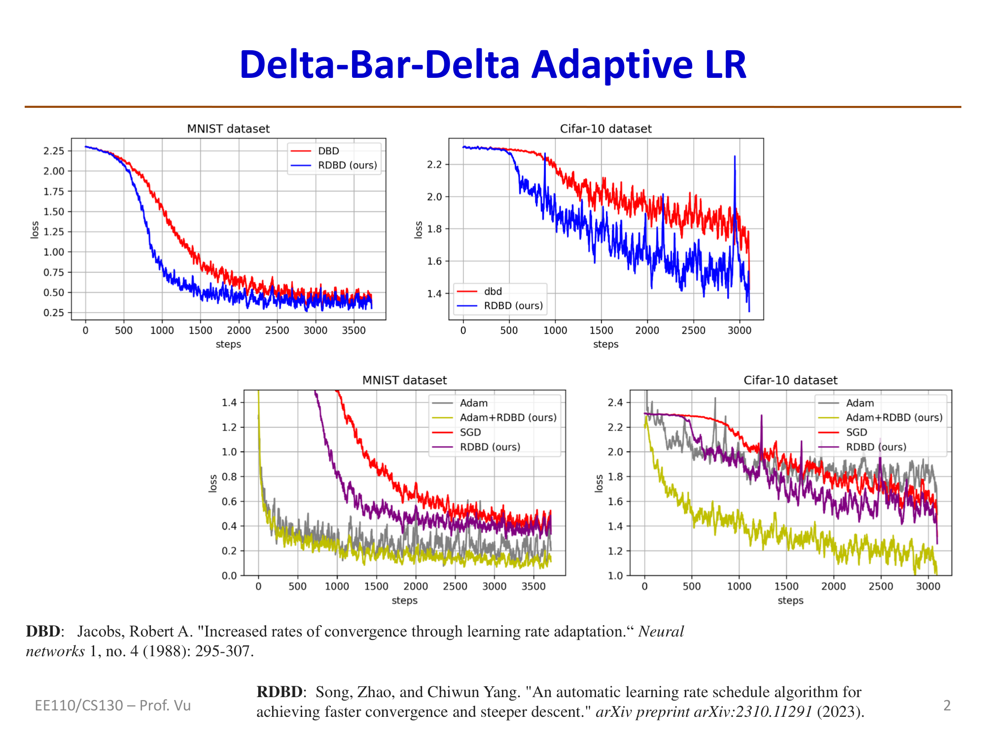
Reference: Song, Zhao, and Chiwun Yang. "An automatic learning rate schedule algorithm for achieving faster convergence and steeper descent." arXiv preprint arXiv:2310.11291 (2023).

---

Optimal Learning Rate and Its Relationship to the Hessian

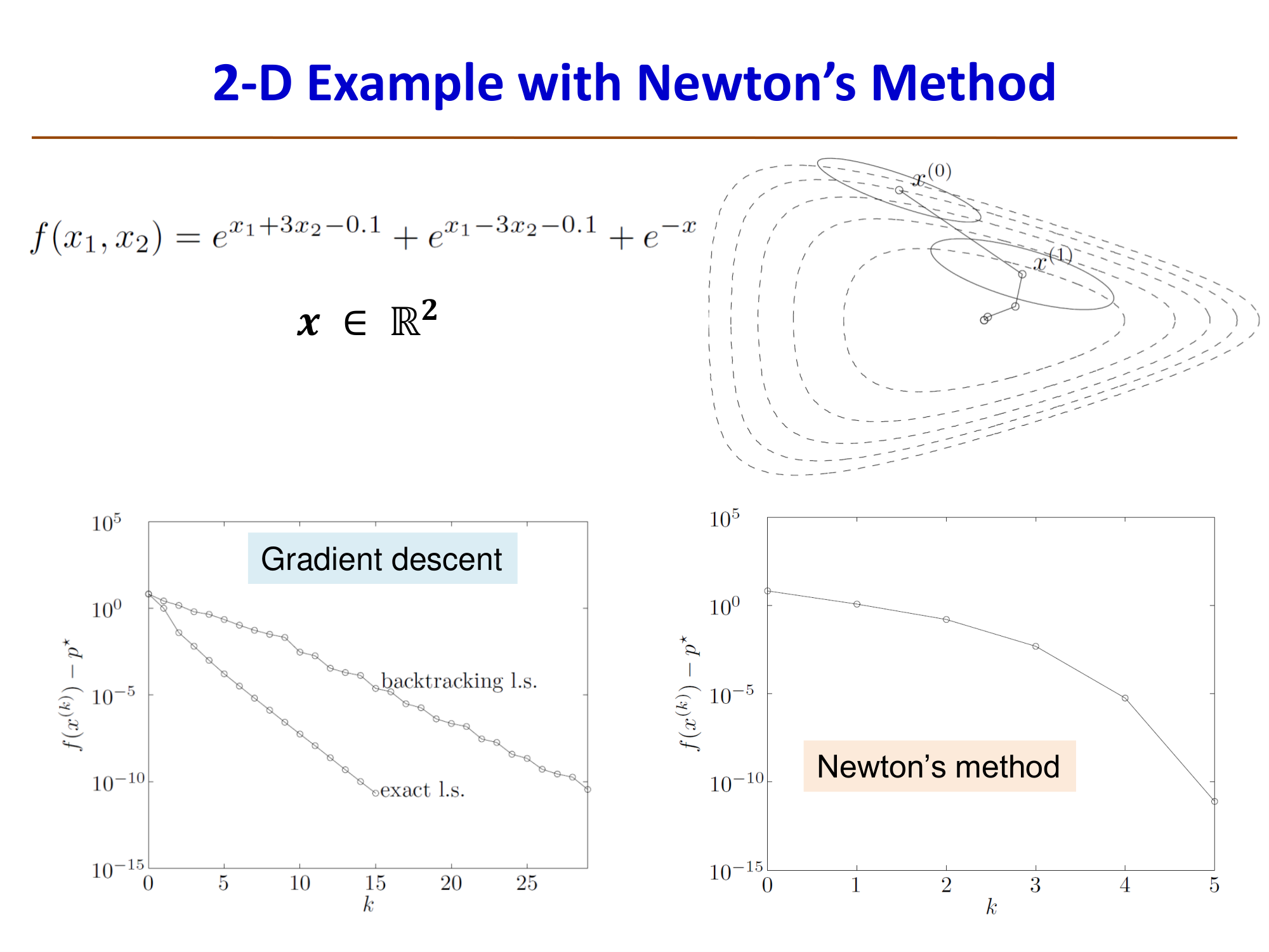
Deriving the Optimal Learning Rate from Newton's Method

Recall that gradient descent uses only the first derivative (gradient): \(\Delta\theta_{GD}^{(k)} = -\nabla J(\theta^{(k)})\), while Newton's method uses the second derivative (Hessian) and converges much faster than GD:

\[ \Delta\theta_{Newton}^{(k)} = -[\nabla^2 J(\theta^{(k)})]^{-1} \cdot \nabla J(\theta^{(k)}) = -H_k^{-1} \cdot g_k \]

where \(H_k = \nabla^2 J(\theta^{(k)})\) is the Hessian matrix (\(n \times n\)).

Intuition in the 1D case: Consider \(\min_\theta f(\theta)\), \(\theta \in \mathbb{R}\). Then:

\[ \Delta\theta_{GD} = -f'(\theta) = -g, \quad \Delta\theta_{Newton} = -(f''(\theta))^{-1} \cdot f'(\theta) = -h^{-1} \cdot g \]

where \(h = f''(\theta)\) is the second derivative. Therefore:

\[ \Delta\theta_{Newton} = \frac{1}{h} \cdot (-g) = \frac{1}{h} \cdot \Delta\theta_{GD} \]

This implies that the optimal learning rate is:

\[ \boxed{\lambda_{opt} = \frac{1}{h}} \]

That is, the learning rate should be the reciprocal of the Hessian (second derivative), which would allow GD to match the performance of Newton's method.

Note: This \(\lambda_{opt} = 1/h\) holds strictly only in the 1D case. In high dimensions, the Newton step involves the full Hessian inverse \(H^{-1}\) and cannot be simply replaced by a scalar learning rate.

Preconditioning

Since computing the full \(H^{-1}\) is extremely expensive (\(n \times n\) matrix inversion), practical methods use a per-dimension approximation: only the diagonal elements of the Hessian are used, applying an independent learning rate to each parameter. This is called preconditioning, and its effect is to stretch or compress certain dimensions so that the loss surface becomes less ill-conditioned.

Notes on Hessian computation:

1. How to compute the Hessian diagonal? Typically by backpropagating through the gradient itself (backprop of backprop), which requires an additional backward pass that can be executed in parallel with the standard backward pass (with a one-step delay).
2. Effect of mini-batches: Due to the use of random data, the resulting Hessian diagonal is an estimate of the true Hessian.

---

AdaDelta

AdaDelta (Zeiler, 2012) leverages the "idea" of the Hessian without explicitly computing second derivatives. Its core derivation is as follows:

Starting from the Newton step: \(\Delta\theta_{Newton} = -g/h\), so \(1/h = -\Delta\theta_{Newton}/g\).

In AdaGrad/RMSProp: \(\Delta x = -\frac{\eta}{\sqrt{v_t + \epsilon}} g_t\), where \(v_t = \beta v_{t-1} + (1-\beta)g_t^2\), giving an effective learning rate \(\lambda_t = \eta / \sqrt{v_t + \epsilon}\).

To make \(\lambda_t \approx 1/h\), i.e., \(\frac{\eta}{\sqrt{v_t + \epsilon}} \approx \frac{\Delta\theta_{Newton}}{g_t}\). Since \(\sqrt{v_t + \epsilon}\) contains gradient information (equivalent to \(g_t\)), we want \(\eta\) to be equivalent to \(\Delta\theta\) -- replacing it with the RMS of past parameter updates:

\[ \eta_t^2 = \text{RMS}(\Delta\theta)_t = \beta \eta_{t-1}^2 + (1-\beta)\Delta\theta_t^2 \]

This yields the AdaDelta update rule:

\[ \lambda_t = -\frac{\text{RMS}(\Delta\theta)_{t-1}}{\text{RMS}(g_t)} \]

\[ \theta^{(t+1)} = \theta^{(t)} - \frac{\eta_t}{\sqrt{v_t + \epsilon}} \cdot g_t \]

where:

\[ \begin{cases} \eta_t^2 = \beta \eta_{t-1}^2 + (1-\beta)\Delta\theta_t^2 \\ v_t = \beta v_{t-1} + (1-\beta)g_t^2 \end{cases} \]

Characteristics: AdaDelta does not require manually setting a global learning rate \(\eta\), which is its main advantage over AdaGrad and RMSProp. However, there are currently no theoretical convergence guarantees.

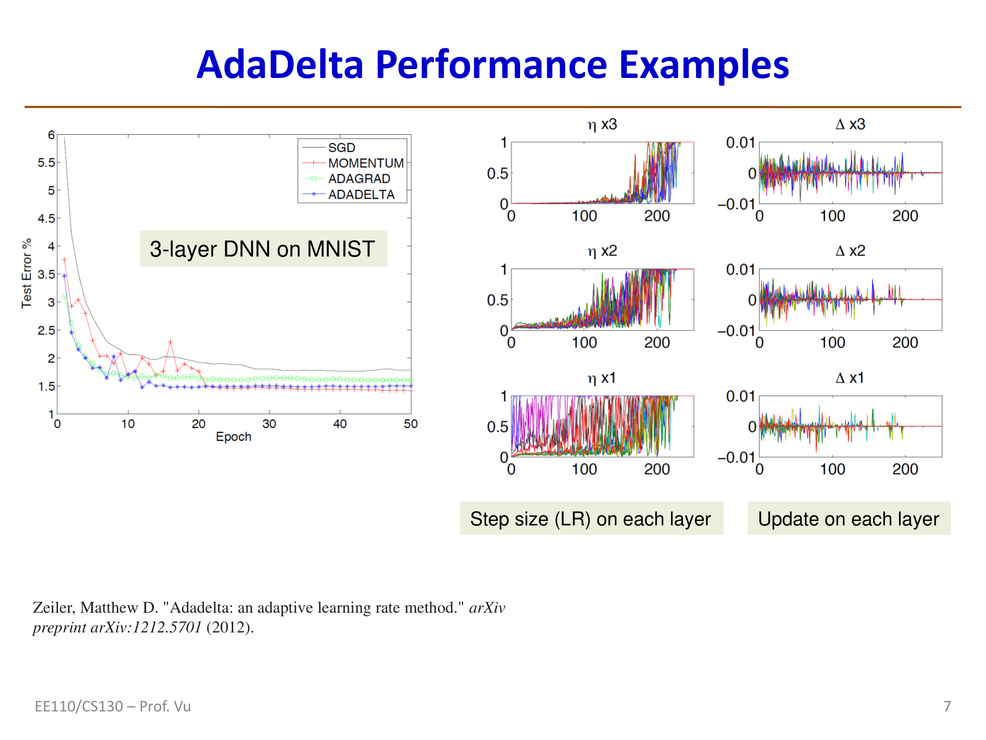
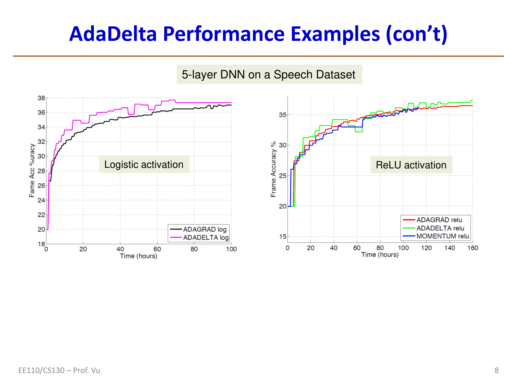
Reference: Zeiler, M. D. "Adadelta: an adaptive learning rate method." arXiv preprint arXiv:1212.5701 (2012).

---

Adaptive Gradient Descent without Descent (AdGD)

Malitsky and Mishchenko (2019) proposed an adaptive learning rate method that does not rely on line search. The core idea is to use the gradient difference between consecutive iterations to approximate the Hessian:

\[ L_k = \frac{\|\nabla J(\theta^k) - \nabla J(\theta^{k-1})\|}{\|\theta^k - \theta^{k-1}\|} \]

Note that \(L_k\) approximates the derivative of the gradient, i.e., it approximates the Hessian \(h_k\). The learning rate is then updated as:

\[ \lambda_k = \min\left\{\sqrt{1 + r_{k-1}} \cdot \lambda_{k-1}, \; \frac{\alpha}{L_k}\right\} \]

where \(r_k = \lambda_k / \lambda_{k-1}\). This formula has two components: \(\sqrt{1 + r_{k-1}} \cdot \lambda_{k-1}\) effectively increases the learning rate, while \(\alpha / L_k\) is an approximation of the Hessian reciprocal.

Theoretical guarantee: For convex loss functions with local smoothness, the convergence rate is \(\|J(\theta^k) - J(\theta^*)\| \sim O(1/k)\).

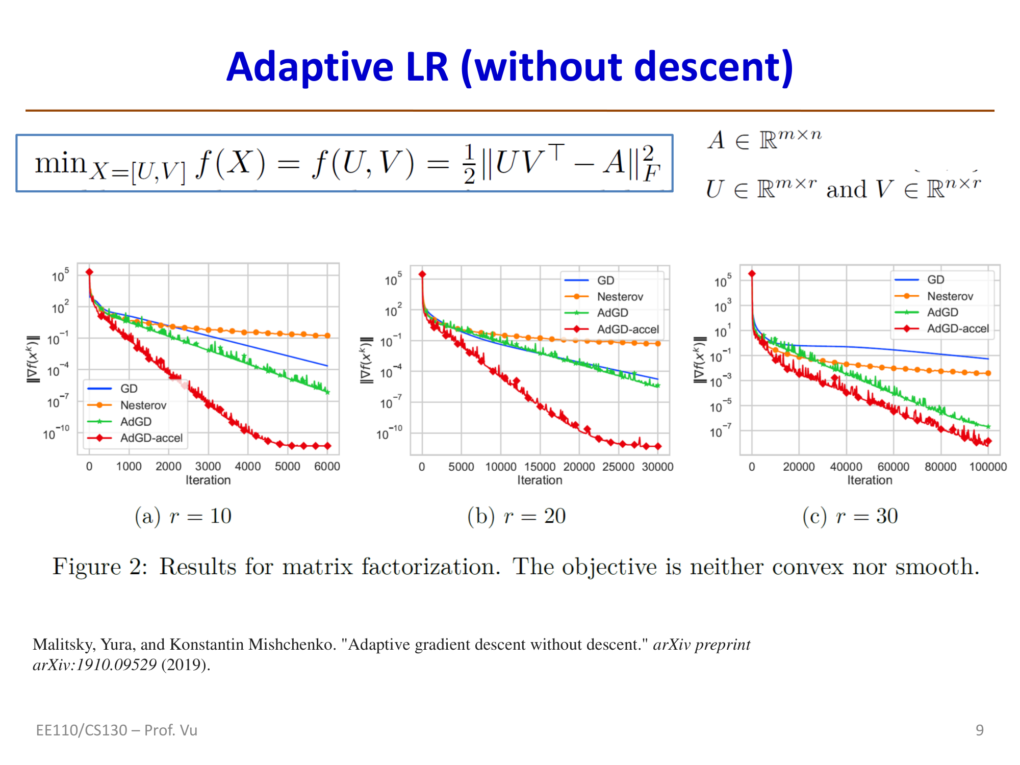
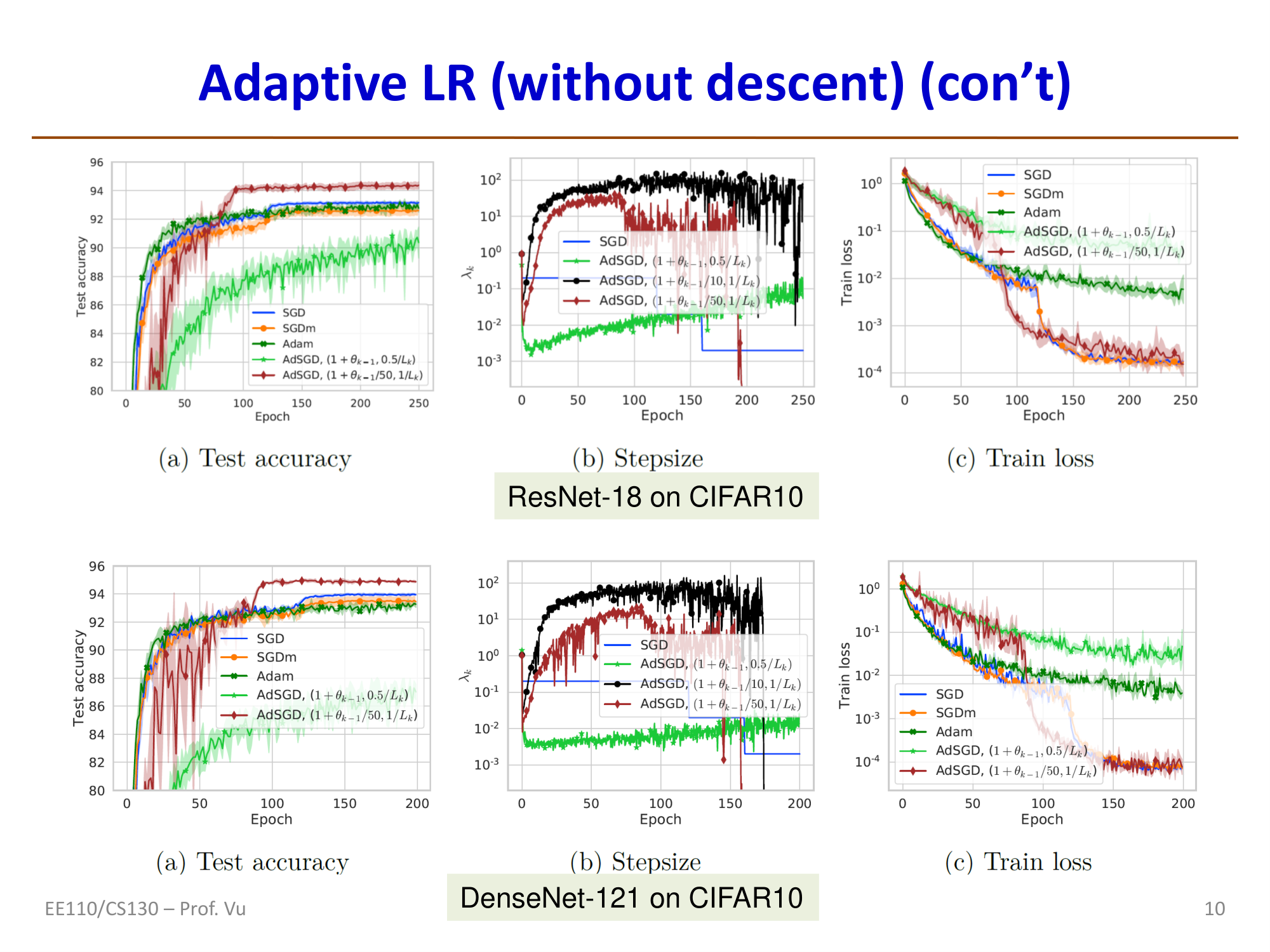
Reference: Malitsky, Y. and Mishchenko, K. "Adaptive gradient descent without descent." arXiv preprint arXiv:1910.09529 (2019).

---

vSGD: Learning Rate Adaptation Based on Second-Order Information

Schaul, Zhang, and LeCun (2013) proposed vSGD, which derives the optimal per-dimension learning rate \(i\) by minimizing the expected loss (accounting for the effect of random data):

\[ \lambda_t^* = \frac{1}{h_i} \cdot \frac{(\theta^{(t)} - \theta^*)^2}{(\theta^{(t)} - \theta^*)^2 + \sigma^2} \]

where \(\sigma^2\) is the variance of the optimal parameters. Since \(\theta^*\) and its variance are unknown in practice, the above is approximated as:

\[ \lambda_i^* = \frac{1}{h_i} \cdot \frac{(\mathbb{E}[g_i])^2}{\mathbb{E}[g_i^2]} = \frac{1}{h_i} \cdot \frac{(\mathbb{E}[g_i])^2}{(\mathbb{E}[g_i])^2 + \text{Var}[g_i]} \]

vSGD algorithm (with exponential moving averages):

\[ \begin{aligned} \bar{g}_i &\leftarrow (1 - \beta_i)\bar{g}_i + \beta_i g_i & \text{(gradient EMA)} \\ \bar{v}_i &\leftarrow (1 - \beta_i)\bar{v}_i + \beta_i g_i^2 & \text{(squared gradient EMA)} \\ \bar{h}_i &\leftarrow (1 - \beta_i)\bar{h}_i + \beta_i |\text{bbprop}(g_i)| & \text{(diagonal Hessian EMA)} \\ \lambda_i &\leftarrow \frac{(\bar{g}_i)^2}{h_i \cdot \bar{v}_i} & \text{(adaptive learning rate)} \\ \frac{1}{\beta_i} &\leftarrow \left(1 - \frac{(\bar{g}_i)^2}{\bar{v}_i}\right)\frac{1}{\beta_i} + 1 & \text{(update forgetting factor)} \\ \theta_i &\leftarrow \theta_i - \lambda_i \cdot \bar{g}_i & \text{(parameter update)} \end{aligned} \]

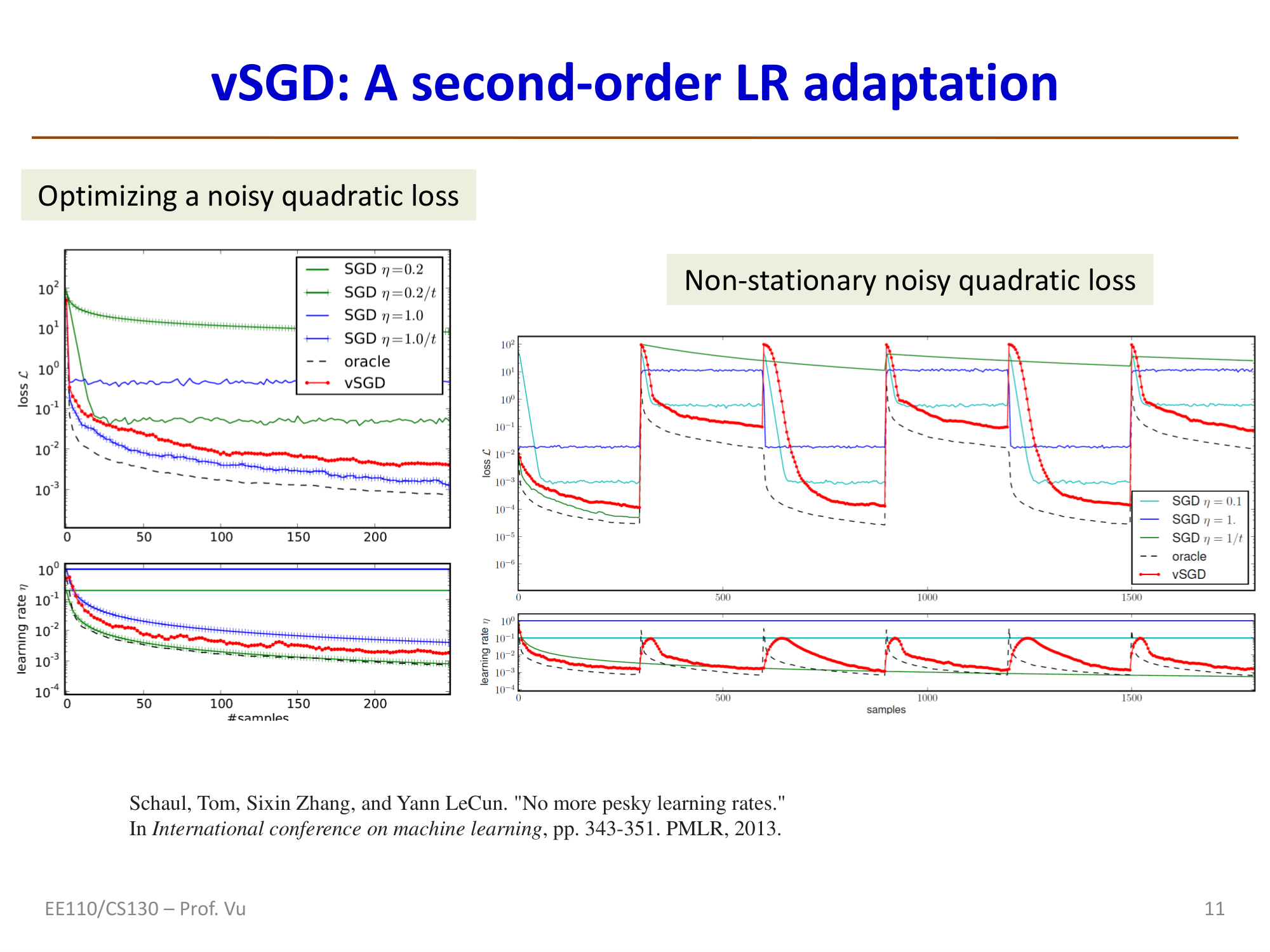
Reference: Schaul, T., Zhang, S., and LeCun, Y. "No more pesky learning rates." ICML, pp. 343-351. PMLR, 2013.

---

---

评论