Algorithm Fundamentals

Basic Data Structures

Before studying algorithms, one should generally have a solid grasp of basic data structures.

Arrays

An Array is the most fundamental linear data structure. It occupies a contiguous block of memory and stores elements of the same type.

Core properties of arrays:

• Fixed size: The length of an array must be specified at creation and cannot change afterward (dynamic arrays such as Python's list automatically resize under the hood, but the underlying mechanism involves creating a new array and copying elements).
• Random Access: Any element can be accessed in \(O(1)\) time via its index, since the address can be computed directly as base_address + index * element_size.
• Contiguous memory: Elements are tightly packed in memory, providing excellent cache locality and efficient traversal.

Operation	Time Complexity	Description
Access	\(O(1)\)	Direct access by index
Search	\(O(n)\)	Linear scan required for unsorted arrays
Insert	\(O(n)\)	Subsequent elements must be shifted
Delete	\(O(n)\)	Subsequent elements must be shifted
Append	\(O(1)\) amortized	Amortized complexity for dynamic arrays

In Python, list is the implementation of a dynamic array:

arr = [1, 2, 3, 4, 5]
print(arr[2])       # O(1) 随机访问，输出 3
arr.append(6)       # O(1) 均摊，尾部追加
arr.insert(0, 0)    # O(n)，头部插入需要移动所有元素

Matrix

A Matrix is essentially a two-dimensional array used to store data in an \(m \times n\) grid. In algorithm problems, matrices are commonly used to represent adjacency relations in graphs, image pixels, dynamic programming state tables, and more.

# 创建 m x n 的矩阵（初始化为0）
m, n = 3, 4
matrix = [[0] * n for _ in range(m)]

# 访问元素：matrix[row][col]，O(1)
matrix[1][2] = 5

Common matrix operations and their complexities:

Operation	Time Complexity	Description
Element access	\(O(1)\)	Direct access by row and column indices
Full matrix traversal	\(O(m \times n)\)	Every element must be visited
Matrix transpose	\(O(m \times n)\)	Swap rows and columns
Matrix multiplication (naive)	\(O(n^3)\)	Multiplying two \(n \times n\) matrices

Common matrix traversal techniques include spiral traversal, diagonal traversal, and level-order traversal (BFS). When working with matrix problems, pay close attention to boundary conditions and the use of direction arrays:

# 四方向移动的方向数组
directions = [(0, 1), (0, -1), (1, 0), (-1, 0)]

for dx, dy in directions:
    nx, ny = x + dx, y + dy
    if 0 <= nx < m and 0 <= ny < n:
        # 处理相邻格子
        pass

Stack

A stack is an abstract data type that follows the Last In, First Out (LIFO) principle. Think of it as a stack of plates: you can only place a plate on top, and you can only take a plate from the top. The last plate placed is the first one removed.

Core operations of a stack:

• Push: Add a new element to the top of the stack.
• Pop: Remove the element from the top of the stack and return its value.
• Peek/Top: Return the value of the top element without removing it.
• isEmpty: Check whether the stack is empty.

Monotonic Stack

A monotonic stack is a special type of stack that maintains the monotonicity of its elements throughout all operations — that is, the elements in the stack are either strictly increasing or strictly decreasing. When a new element \(X\) is about to be pushed, if it would break the stack's monotonicity, all elements at the top that violate the monotonic property must be popped before \(X\) can be pushed, until the stack either satisfies the monotonic property again or becomes empty.

Monotonic stacks are commonly used to solve problems such as:

• Finding the next greater element
• Largest rectangle area

Queue

A Queue is an abstract data type that follows the First In, First Out (FIFO) principle. Think of it as a line at a ticket counter: the first person in line is the first to buy a ticket and leave.

Core operations of a queue:

• Enqueue/Push: Add a new element to the rear of the queue.
• Dequeue/Pop: Remove an element from the front of the queue.
• Peek/Front: Return the value of the front element without removing it.
• isEmpty: Check whether the queue is empty.

Queues have broad applications in computer science, such as:

• Task scheduling: Managing pending tasks or requests in operating systems and servers.
• Breadth-First Search (BFS): Visiting nodes level by level in graph and tree traversals.
• Print job management: Printers typically use a queue to handle pending documents.

Deque

A Deque (Double-Ended Queue) allows enqueue and dequeue operations at both ends (i.e., both the front and the rear).

Monotonic Queue

A monotonic queue is typically implemented using a deque. It leverages the deque's properties to maintain monotonicity, with the primary goal of quickly finding the maximum or minimum value within a sliding window.

• Maintaining monotonicity: When a new element \(X\) is about to be enqueued at the rear, all elements at the rear that violate the monotonic property must be popped.
  • For example, to maintain a decreasing queue (where the front holds the maximum): before enqueuing \(X\), if the rear element \(Y < X\), then \(Y\) is removed. This ensures the queue remains decreasing.
• Handling window sliding: When the sliding window moves to the right, check whether the front element has fallen outside the window. If the front element's index is less than or equal to the current window's starting index, it must be dequeued.
• Retrieving the extremum: Since the queue is monotonic, the front element is always the maximum (for a decreasing queue) or minimum (for an increasing queue) within the current window.

Common applications include:

• Sliding window maximum/minimum
• Dynamic programming optimization

Linked List

A Linked List is a dynamic linear data structure. Unlike arrays, elements in a linked list do not need to be stored contiguously in memory. Each element is called a node, and nodes are connected to the next node via pointers, forming a chain-like structure.

A singly linked list node contains two parts: a data field and a pointer (next) to the next node.

class ListNode:
    def __init__(self, val=0, next=None):
        self.val = val
        self.next = next

Core operations and complexities of linked lists:

Operation	Time Complexity	Description
Access the \(k\)-th element	\(O(n)\)	Must traverse from the head node
Insert/delete at the head	\(O(1)\)	Only the head pointer needs to be modified
Insert at the tail	\(O(n)\)	Must traverse to the tail (without a tail pointer)
Insert/delete after a given node	\(O(1)\)	Only pointers need to be modified
Search	\(O(n)\)	Requires linear traversal

The key difference between linked lists and arrays is: arrays excel at random access in \(O(1)\), while linked lists excel at insertion and deletion in \(O(1)\) (when the position is known). Linked lists do not require pre-allocated space and are well-suited for scenarios with frequent insertions and deletions.

A dummy node (sentinel node) is a commonly used technique in linked list problems. Adding a virtual node before the head unifies the handling of insertions and deletions at the head, avoiding many boundary checks:

def delete_node(head, target):
    dummy = ListNode(0, head)  # 哨兵节点
    prev = dummy
    curr = head
    while curr:
        if curr.val == target:
            prev.next = curr.next  # 删除当前节点
        else:
            prev = curr
        curr = curr.next
    return dummy.next  # 返回真正的头节点

Doubly Linked List

In a Doubly Linked List, each node stores not only its data and a pointer to the next node, but also a pointer to the previous node (prev).

class DoublyListNode:
    def __init__(self, val=0, prev=None, next=None):
        self.val = val
        self.prev = prev
        self.next = next

Compared to singly linked lists, doubly linked lists offer the following advantages:

• Bidirectional traversal: You can traverse forward or backward from any node, whereas a singly linked list only supports forward traversal.
• \(O(1)\) deletion of the current node: In a singly linked list, deleting a node requires knowing its predecessor (which takes \(O(n)\) to find); in a doubly linked list, the predecessor is directly accessible via the prev pointer.
• Core data structure for LRU Cache: A doubly linked list combined with a hash map enables an \(O(1)\) time complexity LRU (Least Recently Used) cache eviction algorithm.

The downside of a doubly linked list is that each node requires an additional prev pointer, resulting in higher space overhead.

Other Data Structures

The following data structures are covered in the Tree algorithm notes:

• Tree
• BST
• Heap
• Fibonacci Heap

The following data structures are covered in the Graph algorithm notes:

• Graph
• Union-Find (DSU)

The following data structures are covered in the String algorithm notes:

• String
• Trie

Algorithm Analysis

Algorithm Analysis Framework

In general, a complete algorithm description typically includes the following components:

• Description
• Pseudocode
• Actual Code
• Justification
• Time Analysis
• Space Analysis

The Description explains the algorithm's content, while the Justification provides correctness proofs or arguments to demonstrate that the analysis results are correct.

For example, for loops in an algorithm, we need to prove the correctness of iterative algorithms. A loop invariant is used to argue that the algorithm does not lose or corrupt key properties during execution.

A loop invariant proof consists of three parts:

• Initialization: Prove that the invariant holds before the first iteration begins.
• Maintenance: Prove that if the invariant holds at the start of some iteration, it still holds at the end of that iteration (i.e., at the start of the next iteration).
• Termination: Prove that when the loop terminates, the invariant provides a useful statement showing that the algorithm's final goal has been achieved.

Beyond loop invariants, time complexity, space complexity, and other claims typically also require justification.

Mathematical Foundations of Algorithm Analysis

This section compiles some mathematical knowledge frequently encountered in this book. These are all relatively basic mathematical concepts.

0.1 Exponential Growth Dominates Polynomial Growth

A critically important rule in algorithm analysis: any exponential function grows faster than any polynomial function.

• Polynomials: Functions of the form \(n^b\), where b is a constant. Examples: \(n^2\), \(n^{100}\).
• Exponentials: Functions of the form \(a^n\), where a is a constant greater than 1. Examples: \(2^n\), \(1.1^n\).

For polynomials and exponentials, if a > 1, we have:

\[ \lim_{n \to \infty} \frac{n^b}{a^n} = 0 \]

This limit formula states that as n approaches infinity, the ratio of a polynomial function to an exponential function approaches 0. This means the denominator grows far faster than the numerator, so in the limit their ratio is essentially 0.

From this, we can derive the following corollary:

\[ n^b = O\!\left(a^n\right) \]

That is, an exponential function is always an upper bound for a polynomial function (when a > 1).

---

0.2 Notation

• \(\log_b n = a \iff b^a = n\) (definition of log)
• \(\ln n = \log_e n\) (natural log)
• \(\lg n \ \text{or} \ \log n = \log_2 n\) (base-2 shorthand)
• \(\lg^2 n = (\lg n)(\lg n)\) (multiplication)
• \(\lg \lg n = (\lg(\lg n))\) (composition)

---

0.3 Notation Properties

• \((a^m)^n = a^{mn}\)
• \(a^m \cdot a^n = a^{m+n}\)
• \(a^n = 2^{n \lg a}\)
• \(a^{\log_b n} = n^{\log_b a}\)
• \(\log_b a = \dfrac{\log_c a}{\log_c b}\) (A way to change from base \(b\) to base \(c\))
• \(\lg ab = \lg a + \lg b\)
• \(\lg(a^x) = x \lg a\)
• \(\lg(1/a) = -\lg a\)

---

0.4 Quantifiers

Quantifiers are used to specify whether a statement holds for every element in a set, or for at least one element.

• Universal Quantifier (\(\forall\)): The symbol \(\forall\) is used to express that a statement holds for every element in a given set. For example:

  $$ \forall x \in \mathbb{R}, \; x^2 \geq 0 $$ - Existential Quantifier (\(\exists\)): The symbol \(\exists\) is used to express that there exists at least one element in a given set for which a statement holds. For example:

  \[ \exists x \in \mathbb{R} \;\; \text{such that} \;\; x^2 = 4 \]

In simple terms:

• ∀ (for all): Has a strict requirement — the statement must hold for every member of the set. The ∀ symbol looks like an upside-down letter "A," which can be associated with the English word "All."
• ∃ (there exists): Has a lenient requirement — only at least one member of the set needs to satisfy the condition. The ∃ symbol looks like a reversed letter "E," which can be associated with the English word "Exists."

These two symbols are essential for defining mathematical concepts (such as the Big O definition discussed earlier) and for constructing logical proofs.

---

0.5 Arithmetic Series Sum Formula

For integer \(n \geq 1\), we have

\[ 1 + 2 + \dots + n \;=\; \sum_{k=0}^n k \;=\; \frac{n(n+1)}{2} \]

---

0.6 Geometric Series Sum Formula

For real \(r \neq 1\), we have

\[ 1 + r + r^2 + \dots + r^k \;=\; \sum_{i=0}^k r^i \;=\; \frac{1 - r^{k+1}}{1-r} \]

When the summation is infinite and \(|r| < 1\), we have

\[ 1 + r + r^2 + \dots \;=\; \sum_{i=0}^{\infty} r^i \;=\; \frac{1}{1-r} \]

---

0.7 Discrete Mathematics and Sets

Let \(A\) and \(B\) be sets.

Union, Intersection, Difference:

• Union: \(A \cup B =\) The set of elements that appear in either \(A\) or \(B\) or both.
• Intersection:\(A \cap B =\) The set of elements that appear in both \(A\) and \(B\).
• Difference:\(A \setminus B\) or \(A - B =\) The set of elements that appear in \(A\) and not in \(B\).

Cardinality (the number of elements in set A):

• Cardinality:\(|A| =\) The number of elements in \(A\).

Factorial:

• Factorial: The notation \(n!\) is read "\(n\) factorial" and is defined for integer \(n > 0\) as follows:

  \[ n! = 1 \times 2 \times \dots \times (n-1) \times n \]

  By convention, \(0! = 1\).

Choose, Permutations, Combinations:

• "Choose": The notation \(\binom{n}{k}\) is read "\(n\) choose \(k\)" because it represents the number of ways to choose \(k\) items from \(n\) distinct items.For integers \(0 \leq k \leq n\), we have:

  $$ \binom{n}{k} = \frac{n!}{k!(n-k)!} = \binom{n}{n-k} $$ - Permutations and Combinations: In a set of elements \(A\), the number of ordered permutations of all \(|A|\) elements is \(|A|!\). The number of combinations of \(k\) elements is

  \[ \binom{|A|}{k}. \]

The most important distinction between permutations and combinations is: order matters in permutations, but not in combinations. For example, ABC and CAB are two different permutations, but they represent the same combination.

---

0.8 Probability

• Random Variables: In probability theory, a random variable is a variable whose possible values are outcomes of a random phenomenon.For example, let \(X\) represent the outcome of rolling a six-sided die.\(X\) can take values \(\{1,2,3,4,5,6\}\).
• Notation:\(P(X = 5) = \tfrac{1}{6}\) means "The probability that \(X\) takes the value \(5\) is \(\tfrac{1}{6}\)."

Expectation:

• Expectation: The expectation (or mean) of a random variable \(X\) is denoted by \(E[X]\) and represents the average value it takes. For a discrete random variable, it is computed as:

  \[ E[X] = \sum_x x \cdot P(X = x) \]

  where the sum is taken over all possible values of \(X\).

Example: Consider a fair six-sided die. Let \(X\) be the outcome of a single roll. The expectation of \(X\) is:

\[ E[X] = \tfrac{1}{6}(1) + \tfrac{1}{6}(2) + \tfrac{1}{6}(3) + \tfrac{1}{6}(4) + \tfrac{1}{6}(5) + \tfrac{1}{6}(6) = \tfrac{7}{2} \]

Properties of Expectation:

• \(E[aX + b] = aE[X] + b\) for constants \(a\) and \(b\).
• \(E[X + Y] = E[X] + E[Y]\) for independent random variables \(X\) and \(Y\).

---

0.9 Ceilings and Floors

• \(\lceil x \rceil = \text{ceiling}(x) =\) the least integer greater than or equal to \(x\)
• \(\lfloor x \rfloor = \text{floor}(x) =\) the greatest integer less than or equal to \(x\)

Complexity Analysis

In algorithm analysis, we use asymptotic notation to analyze the efficiency of algorithms. It encompasses three core concepts:

• Big O
• Big Omega \(\Omega\)
• Big Theta \(\Theta\)

Big O

• Definition: The function \(f(n)\) is \(O(g(n))\) if there exist constants \(c > 0\) and \(n_0\) such that

  $$ 0 \leq f(n) \leq c \cdot g(n) \quad \text{for all } n \geq n_0. $$ - Example: \(2n^2 + 3n + 1\) is \(O(n^2)\) because for \(c = 3\) and \(n_0 = 1\), we have

  \[ 0 \leq 2n^2 + 3n + 1 \leq 2n^2 + 3n^2 + 1 \cdot n^2 \leq 6n^2 , \quad \text{for all } n \geq 1 \]

Generally speaking, Big O describes an upper bound on a function's growth rate. It can be understood as: "When the input size n is sufficiently large, the growth rate of f(n) does not exceed c times that of g(n)."

Typically, \(n_0\) is chosen as 1, or some integer greater than 1. (Although the definition above does not explicitly require \(n_0 \geq 1\), in algorithm analysis we conventionally assume \(n_0 \geq 1\). This is because we care about asymptotic behavior and aim to describe the long-term growth trend of a function, so starting \(n_0\) at a negative value would be meaningless in this context.)

In other words, in algorithm analysis, \(g(n)\) is an upper bound for \(f(n)\), and we do not concern ourselves with constant factors. So when analyzing an algorithm's Big O, we simply need to find appropriate \(c\) and \(n_0\), and identify \(g(n)\).

From a strictly mathematical standpoint, the example above would still be correct if we stated \(O(n^3)\) — it is a valid upper bound, but a very "loose" one that does not accurately reflect the growth trend of \(2n^2\). It is like asking how tall a child is and answering: "They're definitely no taller than 3 meters." While technically correct, this is not very useful. We would rather hear: "They're about 1.2 meters tall." Therefore, when analyzing algorithm complexity, although infinitely many correct Big O answers exist, the convention is to always seek and provide the simplest, tightest one — that is, the smallest growth rate. When a strict upper bound can be established, it is sometimes written using little-o notation.

There are two common ways to write Big O:

• f(n) = O(n²): This is the most common and widely used notation. It reads "f(n) is O of n-squared." Although the equals sign = is used here, it does not denote strict mathematical equality — rather, it is a conventional notation meaning "the growth rate of f(n) belongs to the O(n²) class."
• f(n) ∈ O(n²): This is a more rigorous notation from the set-theoretic perspective. The ∈ symbol means "is an element of." O(n²) actually represents a set of functions — the set of all functions whose growth rate does not exceed n². So f(n) ∈ O(n²) means "f(n) is a member of the set O(n²)."

---

Proving a Big O Property

If f(n) = O(g(n)) and h(n) = O(g(n)), then f(n) + h(n) = O(g(n)).

In plain language: If two functions f(n) and h(n) both grow at most as fast as g(n) (or slower), then their sum f(n) + h(n) also grows at most as fast as g(n).

This is very useful in algorithm analysis. For instance, if you have two sequential code blocks whose running times are O(n) and O(n) respectively, then the overall running time is O(n) + O(n), which by this theorem is still O(n).

PROOF

The proof follows strictly from the definition of Big O notation. Let us proceed step by step:

1. Suppose

Suppose f = O(g) and h = O(g).

The first step is to assume the premises hold. Here we assume f has growth rate O(g), and h also has growth rate O(g). (Note: f is shorthand for f(n), which is common in mathematical proofs.)

2. Expand the definition of f = O(g)

f = O(g) means f ≤ c*g for n ≥ n₀.

This is the formal definition of Big O notation. f(n) = O(g(n)) means: There exists a positive constant c and an integer n₀ such that for all n ≥ n₀, the value of f(n) never exceeds c times the value of g(n).

• c is a constant coefficient that allows us to ignore constant-factor differences.
• n₀ is a threshold indicating that we only care about behavior when the input size n is sufficiently large.

3. Expand the definition of h = O(g)

h = O(g) means h ≤ d*g for n ≥ n₁.

Similarly, h(n) = O(g(n)) means: There exists another positive constant d and another integer n₁ such that for all n ≥ n₁, the value of h(n) never exceeds d times the value of g(n). Note: The constant d and threshold n₁ here may differ from the c and n₀ for f(n).

4. Adding gives

Adding gives f + h ≤ (c+d)g for n ≥ ?

Now, to prove the result for f(n) + h(n), we add the two inequalities: f(n) ≤ c*g(n) h(n) ≤ d*g(n) Adding them yields: f(n) + h(n) ≤ c*g(n) + d*g(n) Factoring out g(n): f(n) + h(n) ≤ (c+d)g(n)

5. Determining the new threshold n The key question is: under what condition does the new inequality f+h ≤ (c+d)g hold?

• The first inequality f ≤ c*g requires n ≥ n₀.
• The second inequality h ≤ d*g requires n ≥ n₁. For both inequalities to hold simultaneously, n must satisfy both n ≥ n₀ and n ≥ n₁. Therefore, we simply take the larger of the two as the new threshold. We define a new threshold n₂ = max(n₀, n₁). When n ≥ n₂, both inequalities hold, and so does their sum.

So the blank in the expression should be filled with max(n₀, n₁).

Conclusion

We have shown that: There exists a new constant C = c+d and a new threshold n₂ = max(n₀, n₁) such that for all n ≥ n₂, f(n) + h(n) ≤ C * g(n).

This perfectly satisfies the definition of Big O notation! Therefore, we conclude: f(n) + h(n) = O(g(n)). QED.

Simple Example

Suppose f(n) = 2n + 10, h(n) = 3n + 5, and we want to prove f(n) + h(n) is O(n).

1. Prove f(n) = O(n): We need to find c and n₀ such that 2n + 10 ≤ c*n. If we choose c = 3, then 2n + 10 ≤ 3n implies 10 ≤ n. So with c₁=3, n₀=10, f(n) = O(n) holds.
2. Prove h(n) = O(n): We need to find d and n₁ such that 3n + 5 ≤ d*n. If we choose d = 4, then 3n + 5 ≤ 4n implies 5 ≤ n. So with c₂=4, n₁=5, h(n) = O(n) holds.
3. Prove f(n) + h(n) = O(n): f(n) + h(n) = (2n+10) + (3n+5) = 5n + 15. By the proof above, we should have f(n) + h(n) ≤ (c₁+c₂)n for n ≥ max(n₀, n₁).

• New constant C = c₁ + c₂ = 3 + 4 = 7.
• New threshold n₂ = max(n₀, n₁) = max(10, 5) = 10.
• Let us verify: does 5n + 15 ≤ 7n hold for n ≥ 10? 15 ≤ 2n implies 7.5 ≤ n. Since n ≥ 10 already satisfies n ≥ 7.5, the inequality holds.

Therefore, we have successfully proved that f(n) + h(n) = O(n).

---

Big Omega

• Definition: The function \(f(n)\) is \(\Omega(g(n))\) if there exist constants \(c > 0\) and \(n_0\) such that

  $$ 0 \leq c \cdot g(n) \leq f(n) \quad \text{for all } n \geq n_0. $$ - Example: \(2n^2 + 3n + 1\) is \(\Omega(n^2)\) because for \(c = 2\) and \(n_0 = 1\), we have

  \[ 0 \leq 2n^2 \leq 2n^2 + 3n + 1, \quad \text{for all } n \geq 1 \]

Generally speaking, Big Omega describes a lower bound on a function's growth rate. It can be understood as: "When the input size n is sufficiently large, the growth rate of f(n) is at least as fast as d times that of g(n)." In other words, g(n) serves as a "floor" for f(n) — no matter how slowly f(n) grows, it cannot grow slower than g(n). In algorithm analysis, it is commonly used to describe the best-case time complexity of an algorithm.

For any growing function f(n) (such as an algorithm's running time), we can almost always say f(n) = Ω(1) (since running time is at least a constant and cannot be negative). However, this is an uninformative "loose" lower bound.

We use Big Omega to answer the question: "How fast must this algorithm's running time grow at minimum?" Saying Ω(1) is equivalent to saying: "This algorithm takes some time to run." That is a trivially obvious statement. Saying a sorting algorithm is Ω(n) means: "No matter how favorable the input data is (e.g., already sorted), you must look at each element at least once, so the time lower bound is linear growth." This is genuinely useful information.

Therefore, in practice, just as with Big O, we seek the tightest lower bound — the fastest-growing lower bound function — to provide a meaningful analysis. When a strict lower bound can be established, it is denoted using little-omega notation (\(\omega\)).

---

Big Theta

• Definition: The function \(f(n)\) is \(\Theta(g(n))\) if it is both \(O(g(n))\) and \(\Omega(g(n))\).
• Example: \(2n^2 + 3n + 1\) is \(\Theta(n^2)\) because it is both \(O(n^2)\) and \(\Omega(n^2)\).

f(n) = Θ(g(n)) means: there exist positive constants c, d, and n₀ such that for all n ≥ n₀, we have d * g(n) ≤ f(n) ≤ c * g(n). Big Theta describes a tight bound on a function's growth rate. It is essentially the combination of Big O and Big Omega. f(n) = Θ(g(n)) means f(n) grows neither faster nor slower than g(n) — their growth rates are identical. In other words, f(n) is "sandwiched" by g(n) from both above and below. This is the most precise description of an algorithm's complexity.

Generally, if when seeking Big O and Big Omega we already find the tightest upper bound and the tightest lower bound, we can easily identify the tight bound that is sandwiched between them.

Recursion

Recursion

Recursion is a method of solving problems. In computer science, when a function calls itself within its own body, it forms recursion.

For example:

def factorial(n):
    # 递归终止条件（基例）
    if n == 1:
        return 1
    # 递归调用
    return n * factorial(n - 1)

print(factorial(5))  # 输出：120

Its working principle is as follows:

factorial(5)
= 5 * factorial(4)
= 5 * (4 * factorial(3))
= 5 * (4 * (3 * factorial(2)))
= 5 * (4 * (3 * (2 * factorial(1))))
= 5 * 4 * 3 * 2 * 1
= 120

Internally, recursion relies on the runtime stack (also known as the call stack). Each time a function is called (whether calling another function or itself), the computer must record the current function's execution context so that it can return correctly after the function completes. This mechanism is implemented via the stack.

Since the underlying implementation uses a stack, we can of course use an explicit stack data structure to achieve the same effect. In computer science, any recursive algorithm can theoretically be converted into an equivalent iterative algorithm whose core is an explicitly managed stack.

The factorial example above, rewritten with an explicit stack:

def factorial_stack(n):
    stack = []      # 用来模拟递归调用栈
    result = 1

    # 模拟递归"向下调用"的过程
    while n > 1:
        stack.append(n)
        n -= 1

    # 模拟递归"向上返回"的过程
    while stack:
        result *= stack.pop()

    return result

print(factorial_stack(5))  # 输出：120

The advantage of using an explicit stack is that the available space is far greater than the system call stack, enabling the handling of deeper, larger-scale recursive problems. Additionally, explicit stacks offer better performance, so when we later encounter recursive algorithms like DFS, they almost always have corresponding iterative versions that are very common in practice.

It is important to note that from the perspective of computer execution and code implementation, the iterative version is not recursion since it does not use the function call stack. However, from the perspective of algorithm design philosophy and problem decomposition, the iterative implementation is still an application of recursive thinking.

Divide and Conquer

Divide and conquer means "divide and rule." Divide and conquer always involves recursion, but recursion is not always divide and conquer. The core idea of divide and conquer is to break a large problem into several smaller subproblems, solve them recursively, and then combine their solutions to obtain the solution to the original problem.

Divide and conquer typically involves three steps:

1. Divide: Decompose the original problem into \(k\) smaller subproblems. These subproblems are usually independent and have the same form as the original problem.
2. Conquer: If a subproblem is small enough (reaching the base case), solve it directly. Otherwise, continue recursively applying the divide and conquer process.
3. Combine: Merge the solutions of the subproblems to form the final solution of the original problem. This "combine" step is often the most ingenious and critical part of a divide and conquer algorithm.

Divide and conquer is widely used in many efficient algorithms, such as:

Merge Sort

• Divide: Split the array to be sorted into two sub-arrays (left and right).
• Conquer: Recursively sort these two sub-arrays.
• Combine: Merge the two sorted sub-arrays into a single sorted array.

Quick Sort

• Divide: Choose a pivot element, then partition the array into two parts via a single scan: elements smaller than the pivot and elements greater than the pivot.
• Conquer: Recursively sort both parts.
• Combine: Since the partition operation has already placed elements in their correct relative positions, the combine step is trivial (just concatenate the two parts with the pivot, or equivalently, the merge cost is virtually zero).

Binary Search

• Divide: Split the search interval in half.
• Conquer: Based on the comparison between the target value and the middle element, recursively search in only one half of the interval.
• Combine: If found, return the index; if not found, return a not-found signal (no actual merge operation).

Strassen Matrix Multiplication

• Divide: Partition an \(N \times N\) matrix into four \((N/2) \times (N/2)\) sub-matrices.
• Conquer: Recursively compute seven \((N/2) \times (N/2)\) matrix multiplications (instead of the traditional eight).
• Combine: Through addition and subtraction of these seven results, compose the final \(N \times N\) matrix product.

Recurrence Relations

The running time \(T(n)\) of recursive or divide-and-conquer algorithms is typically described and analyzed using recurrence relations. For a typical divide-and-conquer algorithm:

1. Cost of divide and combine: \(f(n)\)
2. Number of subproblems: \(a\)
3. Subproblem size: \(n/b\)

The recurrence relation for the running time is generally written as:

\[ T(n) = aT(n/b) + f(n) \]

For example, the recurrence for merge sort is \(T(n) = 2T(n/2) + O(n)\), where \(a=2\) (two subproblems), \(b=2\) (size halved), and \(f(n)=O(n)\) (merge cost). Solving this recurrence yields a time complexity of \(O(n \log n)\) for merge sort.

The purpose of writing a recurrence relation is to analyze time complexity. Computer scientists have developed several powerful tools for quickly solving recurrence relations. The most commonly used methods include:

• Master Theorem
• Recursion-Tree Method
• Substitution Method

Master Theorem

The Master Theorem (or Master Method) is a tool for quickly solving recurrence relations of a specific form:

\[ T(n) = aT\!\left(\tfrac{n}{b}\right) + f(n) \]

where \(a \ge 1\), \(b > 1\) are constants, and \(f(n)\) is an asymptotically positive function:

• \(a\): Number of subproblems
• \(n/b\): Size of each subproblem (assuming equal sizes)
• \(f(n)\): Time spent on dividing the problem and combining subproblem solutions (the non-recursive part)

The core idea of the Master Method is to compare \(f(n)\) with \(n^{\log_b a}\) asymptotically, and then determine the solution for \(T(n)\):

Relationship	Case Description	Conclusion
Case 1	\(f(n) = O(n^{\log_b a - \epsilon})\) (\(n^{\log_b a}\) dominates, by a polynomial factor)	\(T(n) = \Theta(n^{\log_b a})\)
Case 2	\(f(n) = \Theta(n^{\log_b a})\) (\(n^{\log_b a}\) and \(f(n)\) are equal)	\(T(n) = \Theta(n^{\log_b a} \log n)\)
Case 3	\(f(n) = \Omega(n^{\log_b a + \epsilon})\) (\(n^{\log_b a}\) is smaller, by a polynomial factor)	\(T(n) = \Theta(f(n))\)

Note: \(\epsilon\) is a constant greater than 0.

---

Here are several examples illustrating how to apply the Master Method:

a.

\[ T(n) = 2T\!\left(\tfrac{n}{4}\right) + 1 \]

1. Analysis:

   • \(f(n) = 1\)
   • Compare \(f(n) = 1\) with \(n^{\log_b a} = \sqrt{n}\).
   • Clearly, \(f(n)\) grows much slower than \(\sqrt{n}\). Formally, \(f(n) = 1 = O(n^{0.5 - \varepsilon})\); for example, we can take \(\varepsilon = 0.5\).
   • This matches Case 1 of the Master Method. 2. Conclusion:
   • The total cost is dominated by \(n^{\log_b a}\).
   • \[ T(n) = \Theta\!\bigl(n^{\log_b a}\bigr) = \Theta(\sqrt{n}) \]

---

b.

\[ T(n) = 2T\!\left(\tfrac{n}{4}\right) + \sqrt{n} \]

1. Analysis:

   • \(f(n) = \sqrt{n}\)
   • Compare \(f(n) = \sqrt{n}\) with \(n^{\log_b a} = \sqrt{n}\).
   • They are asymptotically equal. Formally, \(f(n) = \Theta\!\bigl(n^{1/2}\log^0 n\bigr)\), i.e., \(k = 0\).
   • This matches Case 2 of the Master Method. 2. Conclusion:
   • The total cost requires an additional logarithmic factor on top of the base.
   • \[ T(n) = \Theta\!\bigl(n^{\log_b a}\log^{k+1} n\bigr) = \Theta\!\bigl(\sqrt{n}\log^{0+1} n\bigr) = \Theta\!\bigl(\sqrt{n}\lg n\bigr) \]

---

c.

\[ T(n) = 2T\!\left(\tfrac{n}{4}\right) + \sqrt{n}\,\lg^{2}n \]

1. Analysis:

   • \(f(n) = \sqrt{n}\,\lg^2 n\)
   • Compare \(f(n) = \sqrt{n}\,\lg^2 n\) with \(n^{\log_b a} = \sqrt{n}\).
   • \(f(n)\) grows faster than \(n^{\log_b a}\), but only by a logarithmic factor (\(\lg^2 n\)), not a polynomial factor. Therefore, it does not satisfy the condition for Case 3.
   • Looking at the generalized form of Case 2: \(f(n) = \Theta\!\bigl(n^{\log_b a}\log^k n\bigr)\).
   • Here, \(f(n) = \Theta\!\bigl(\sqrt{n}\log^2 n\bigr)\), i.e., \(k = 2\).
   • This still matches Case 2 of the Master Method. 2. Conclusion:
   • The total cost requires an additional logarithmic factor.
   • \[ T(n) = \Theta\!\bigl(n^{\log_b a}\log^{k+1} n\bigr) = \Theta\!\bigl(\sqrt{n}\log^{2+1} n\bigr) = \Theta\!\bigl(\sqrt{n}\lg^3 n\bigr) \]

---

d.

\[ T(n) = 2T\!\left(\tfrac{n}{4}\right) + n \]

1. Analysis:

   • \(f(n) = n\)
   • Compare \(f(n) = n\) with \(n^{\log_b a} = \sqrt{n}\).
   • \(f(n)\) grows much faster than \(\sqrt{n}\). Formally, \(f(n) = n^1 = \Omega(n^{0.5+\varepsilon})\); we can take \(\varepsilon = 0.5\).
   • This satisfies the first condition of Case 3 of the Master Method.
   • We also need to check the regularity condition: \(a f(n/b) \leq c f(n)\) for some \(c < 1\).
     • \(2 \cdot f(n/4) \leq c \cdot n\)
     • \(2 \cdot (n/4) \leq c \cdot n\)
     • \(n/2 \leq c \cdot n\)
     • \(1/2 \leq c\)
   • We can choose \(c = 1/2\) (or \(0.6, 0.9\), etc.), which satisfies \(1/2 \leq c < 1\). So the regularity condition holds. 2. Conclusion:
   • The total cost is dominated by \(f(n)\).
   • \[ T(n) = \Theta(f(n)) = \Theta(n) \]

---

e.

\[ T(n) = 2T\!\left(\tfrac{n}{4}\right) + n^2 \]

1. Analysis:

   • \(f(n) = n^2\)
   • Compare \(f(n) = n^2\) with \(n^{\log_b a} = \sqrt{n}\).
   • \(f(n)\) grows much faster than \(\sqrt{n}\). Formally, \(f(n) = n^2 = \Omega(n^{0.5+\varepsilon})\); we can take \(\varepsilon = 1.5\).
   • This also satisfies the first condition of Case 3 of the Master Method.
   • Checking the regularity condition: \(a f(n/b) \leq c f(n)\) for some \(c < 1\).
     • \(2 \cdot f(n/4) \leq c \cdot n^2\)
     • \(2 \cdot (n/4)^2 \leq c \cdot n^2\)
     • \(2 \cdot (n^2/16) \leq c \cdot n^2\)
     • \(n^2/8 \leq c \cdot n^2\)
     • \(1/8 \leq c\)
   • We can choose \(c = 1/8\) (or \(0.5, 0.9\), etc.), which satisfies \(1/8 \leq c < 1\). So the regularity condition holds. 2. Conclusion:
   • The total cost is dominated by \(f(n)\).
   • \[ T(n) = \Theta(f(n)) = \Theta(n^2) \]

.

Recursion-Tree Method

For recurrence relations that do not satisfy the conditions of the Master Theorem, the recursion-tree method can be attempted.

Here is a generalized summary of the recursion-tree method. For a recurrence of the form:

\[ T(n) = A \cdot T\left(\frac{n}{B}\right) + w(n) \]

Symbol	Meaning
\(A\)	Number of subproblems generated at each level of recursion
\(B\)	Reduction factor of each subproblem's size relative to the original
\(w(n)\)	Work done in the divide and combine phases (non-recursive part)

For Level 0 (the root node), there is 1 node and the work done is \(w(n)\).

For Level i (any level), there are \(A^i\) nodes, each with size \(n/B^i\), each doing \(w(n/B^i)\) work. The total work at level \(i\), denoted \(C_i\), is:

\[ C_i = (\text{number of nodes}) \times (\text{work per node}) = A^i \cdot w\left(\frac{n}{B^i}\right) \]

The tree height \(h\) is determined by the condition that recursion terminates when the subproblem size reaches the base case, i.e., size \(1\). Setting \(n/B^h = 1\), we get:

\[ B^h = n \implies h = \log_B n \]

Next, determine the number of leaves. If all leaves are at height \(h\), then the number of leaf nodes equals \(A\) raised to the power \(h\):

\[ \text{Number of leaves} = A^h = A^{\log_B n} \]

Using the change-of-base identity \(a^{\log_b c} = c^{\log_b a}\):

\[ \text{Number of leaves} = n^{\log_B A} \]

The total leaf cost is expressed as \(\Theta(\text{number of leaves} \times \text{base case cost})\). If the base case cost is \(\Theta(1)\), then:

\[ \text{Total leaf cost} = \Theta(n^{\log_B A}) \]

Finally, compute the total work \(T(n)\). The total work is the sum of work across all non-leaf levels, plus the total leaf cost:

\[ \text{Total work } T(n) = \sum_{i=0}^{h-1} (\text{Level } i \text{ total cost}) + (\text{Total leaf cost}) \]

That is:

\[ T(n) = \underbrace{\sum_{i=0}^{\log_B n - 1} A^i \cdot w\left(\frac{n}{B^i}\right)}_{\text{Sum of non-leaf node work}} + \underbrace{\Theta(n^{\log_B A})}_{\text{Total leaf cost}} \]

Compare the contributions from the left and right parts of the expression above; whichever term dominates determines the final time complexity. This generalized framework is the theoretical foundation behind the Master Method. When \(w(n)\) is a polynomial, we can directly use the three cases of the Master Method to avoid complex summation calculations.

---

Example

Let us use the recurrence for QuickSort as an example of how to apply the recursion-tree method.

For the recurrence:

\[ T(n) = T\left(\frac{n}{4}\right) + T\left(\frac{3n}{4}\right) + \Theta(n) \]

The Master Method requires all subproblems to have the same size, i.e., the form \(T(n) = aT(n/b) + f(n)\). In this recurrence, the subproblem sizes are \(n/4\) and \(3n/4\), which are unequal. The recursion tree is a general visualization method particularly suited for recurrences with unequal subproblem sizes; it clearly displays the work at each level and the height of the tree. Therefore, we use the recursion tree to analyze this recurrence.

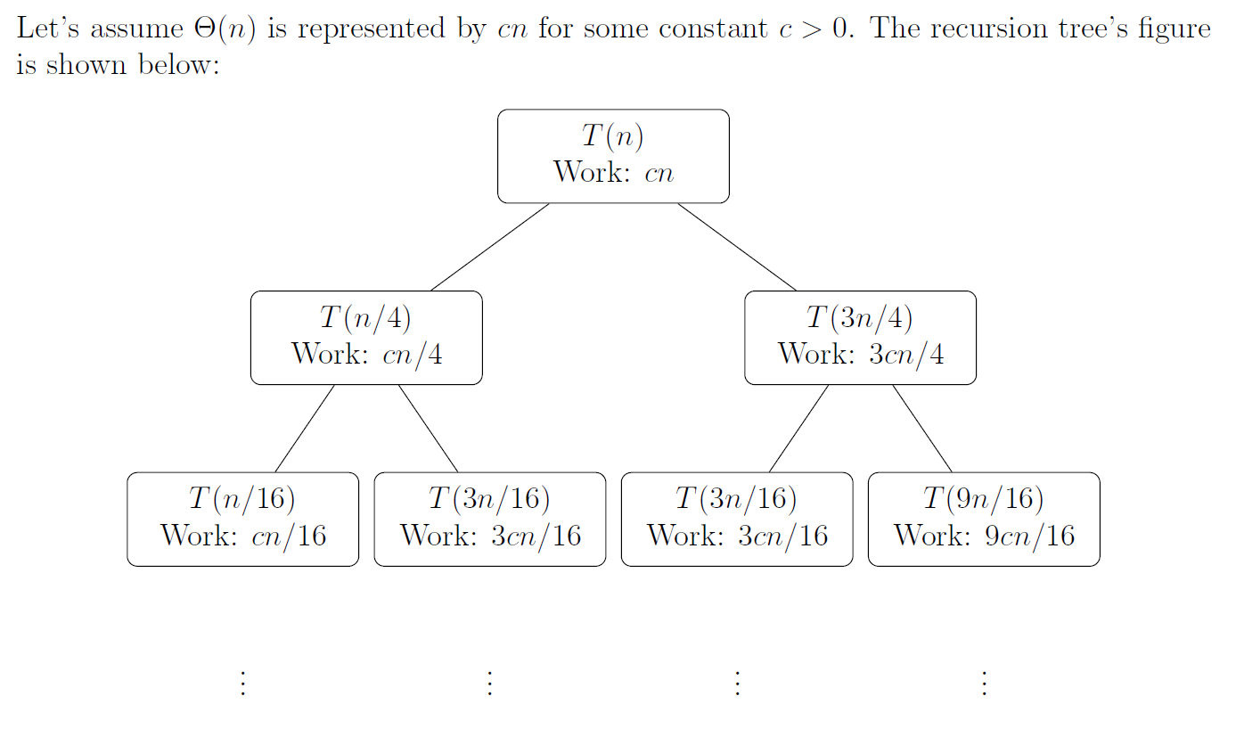
As can be seen, the recursion tree is unbalanced. The two recursive calls \(T(n/4)\) and \(T(3n/4)\) produce subproblems of unequal size:

• The \(T(n/4)\) branch reduces problem size faster.
• The \(T(3n/4)\) branch reduces problem size more slowly, thus forming a deeper path.

We can analyze the shortest path, longest path, and total tree height.

Shortest Path (Shortest Depth): Determined by the fastest-shrinking branch \(T(n/4)\). The shortest depth \(k_{shortest}\) is the depth at which the problem size reaches the base case (e.g., 1).

\[ \frac{n}{4^{k_{shortest}}} = 1 \implies k_{shortest} = \log_4 n \]

Longest Path (Height): Determined by the slowest-shrinking branch \(T(3n/4)\). The longest depth \(k_{longest}\) is the depth at which the problem size reaches the base case (e.g., 1).

\[ \left(\frac{3}{4}\right)^{k_{longest}} n = 1 \implies k_{longest} = \log_{4/3} n \]

Total tree height: \(h = \Theta(\log n)\) (since both \(\log_{4/3} n\) and \(\log_4 n\) belong to \(\Theta(\log n)\))

---

Work at each complete level:

• Level 0 (root): Cost is \(cn\).
• Level 1: Subproblem sizes are \(n/4\) and \(3n/4\).
  • Total cost: \(c\left(\frac{n}{4}\right) + c\left(\frac{3n}{4}\right) = c\left(\frac{n}{4} + \frac{3n}{4}\right) = c n\).
• Level 2: Subproblem sizes are \(n/16, 3n/16, 3n/16, 9n/16\).
  • Total cost: \(c\left(\frac{n}{16}\right) + c\left(\frac{3n}{16}\right) + c\left(\frac{3n}{16}\right) + c\left(\frac{9n}{16}\right) = c\left(\frac{1+3+3+9}{16}\right)n = c\left(\frac{16}{16}\right)n = c n\).
• Observed pattern: At all complete levels, the work is always \(\mathbf{cn}\) or \(\mathbf{\Theta(n)}\).

Formal Justification:

For any level \(i\) (from \(i=0\) to the shortest depth \(\log_4 n\)), the sum of subproblem sizes across all nodes at that level is always \(n\).

A node at level \(i\) is produced by \(j\) splits of \(n/4\) and \(i-j\) splits of \(3n/4\) from root to that node. Its problem size is \(\left(\frac{1}{4}\right)^j \left(\frac{3}{4}\right)^{i-j} n\).

The work at level \(i\), \(\text{Cost}_{\text{level } i}\), is the sum of all node costs:

\[ \text{Cost}_{\text{level } i} = \sum_{j=0}^{i} \begin{pmatrix} i \\ j \end{pmatrix} \cdot c \cdot \left(\frac{1}{4}\right)^j \left(\frac{3}{4}\right)^{i-j} n \]

Factoring out \(cn\):

\[ \text{Cost}_{\text{level } i} = c n \sum_{j=0}^{i} \begin{pmatrix} i \\ j \end{pmatrix} \left(\frac{1}{4}\right)^j \left(\frac{3}{4}\right)^{i-j} \]

By the binomial theorem \(\sum_{j=0}^{i} \begin{pmatrix} i \\ j \end{pmatrix} x^j y^{i-j} = (x+y)^i\), with \(x=1/4\) and \(y=3/4\):

\[ \text{Cost}_{\text{level } i} = c n \left(\frac{1}{4} + \frac{3}{4}\right)^i = c n \cdot (1)^i = \mathbf{cn} \]

This confirms that at all complete levels, the total work is always \(cn\) or \(\mathbf{\Theta(n)}\).

---

Guess:

• Work per level: \(\Theta(n)\)
• Number of levels / height: \(\Theta(\log n)\) (determined by the longest path \(\log_{4/3} n\))
• Total work: (work per level) \(\times\) (number of levels) \(\approx \Theta(n) \times \Theta(\log n) = \mathbf{\Theta(n \log n)}\)

1. Proving the upper bound \(O(n \log n)\)****

Goal: Prove that \(T(n) \le c_2 n \log n\) holds for constants \(c_2 > 0\) and \(n_0\).

Inductive hypothesis: Assume for all \(k < n\), \(T(k) \le c_2 k \log k\) holds.

Substitution and derivation:

\[ T(n) = T\left(\frac{n}{4}\right) + T\left(\frac{3n}{4}\right) + \Theta(n) \]

\[ \le c_2 \left(\frac{n}{4}\right) \log \left(\frac{n}{4}\right) + c_2 \left(\frac{3n}{4}\right) \log \left(\frac{3n}{4}\right) + d_2 n \]

\[ \le c_2 \frac{n}{4} (\log n - \log 4) + c_2 \frac{3n}{4} (\log n - \log (4/3)) + d_2 n \]

\[ \text{（简化，使用 } \log 4 = 2 \text{ 和 } \log (4/3) \approx 0.415 \text{）} \]

\[ = c_2 \log n \left(\frac{n}{4} + \frac{3n}{4}\right) - c_2 n \left(\frac{2}{4} + \frac{3}{4} \log (4/3)\right) + d_2 n \]

\[ = c_2 n \log n - c_2 n \left(\frac{1}{2} + \frac{3}{4} (2 - \log_2 3)\right) + d_2 n \]

\[ = c_2 n \log n - n \left[c_2 \left(\frac{1}{2} + \frac{3}{4} (2 - \log_2 3)\right) - d_2\right] \]

Verification:

For \(T(n) \le c_2 n \log n\) to hold, we need the subtracted term to be non-negative:

\[ n \left[c_2 \left(\frac{1}{2} + \frac{3}{4} (2 - \log_2 3)\right) - d_2\right] \ge 0 \]

\[ \implies c_2 \left(\frac{1}{2} + \frac{3}{4} (2 - \log_2 3)\right) - d_2 \ge 0 \]

The term in parentheses is a positive constant (approximately 0.811). Therefore, we can always choose a sufficiently large constant \(c_2\) (specifically, \(c_2 \ge d_2 / 0.811\)) to satisfy this inequality.

Therefore, the upper bound \(O(n \log n)\) holds.

2. Proving the lower bound \(\Omega(n \log n)\)****

Goal: Prove that \(T(n) \ge c_1 n \log n\) holds for constants \(c_1 > 0\) and \(n_0\).

Inductive hypothesis: Assume for all \(k < n\), \(T(k) \ge c_1 k \log k\) holds.

Substitution and derivation:

\[ T(n) = T\left(\frac{n}{4}\right) + T\left(\frac{3n}{4}\right) + \Theta(n) \]

\[ \ge c_1 \left(\frac{n}{4}\right) \log \left(\frac{n}{4}\right) + c_1 \left(\frac{3n}{4}\right) \log \left(\frac{3n}{4}\right) + d_1 n \]

\[ \text{（使用与上界证明相似的代数简化）} \]

\[ = c_1 n \log n - n \left[c_1 \left(\frac{1}{2} + \frac{3}{4} (2 - \log_2 3)\right) - d_1\right] \]

\[ = c_1 n \log n - c_1 n \left(\frac{1}{2} + \frac{3}{4} (2 - \log_2 3)\right) + d_1 n \]

Verification:

For \(T(n) \ge c_1 n \log n\) to hold, we need the subtracted term to be non-positive:

\[ c_1 n \left(\frac{1}{2} + \frac{3}{4} (2 - \log_2 3)\right) - d_1 n \le 0 \]

\[ \implies c_1 \left(\frac{1}{2} + \frac{3}{4} (2 - \log_2 3)\right) - d_1 \le 0 \]

The term in parentheses is still a positive constant (approximately 0.811). Therefore, we can always choose a sufficiently small positive constant \(c_1\) (specifically, \(0 < c_1 \le d_1 / 0.811\)) to satisfy this inequality.

Therefore, the lower bound \(\Omega(n \log n)\) holds.

Since we have successfully proved both the upper bound \(T(n) = O(n \log n)\) and the lower bound \(T(n) = \Omega(n \log n)\), we conclude the tight bound is:

\[ \mathbf{T(n) = \Theta(n \log n)} \]

This shows that even when Quicksort's pivot selection is unbalanced (e.g., an \(n/4\) vs \(3n/4\) split), its asymptotic running time remains consistent with a balanced split (e.g., \(n/2\) vs \(n/2\)) or the average case of \(\Theta(n \log n)\).

Substitution Method

The substitution method is the most rigorous solving technique. It can be used to verify solutions guessed by other methods and is applicable to all recurrence relations.

However, the substitution method requires an initial guess for the recurrence. Typically, we draw a recursion tree to inform a better guess. After guessing, we use mathematical induction to prove the guess is correct:

1. Inductive hypothesis: Assume for all \(m < n\), \(T(m) \le c g(m)\) holds (where \(c\) is a constant).
2. Proof: Substitute the inductive hypothesis into the original recurrence and show that \(T(n) \le c g(n)\) also holds.
3. Check the base case: Ensure the base case (e.g., \(T(1)\)) also satisfies the hypothesis.

The substitution method is generally used for complex cases where the Master Theorem and the recursion-tree method cannot handle. In practice, we typically try the Master Theorem first. If the Master Theorem does not apply, we use the recursion-tree method to guess the solution, then use the substitution method for a rigorous proof.

---

Worked Examples

a.

\[ T(n) = T(n-1) + n \quad \Rightarrow \quad T(n) = O(n^2) \]

1. State the goal: We want to prove \(T(n) = O(n^2)\). By definition, we need to find constants \(c > 0\) and \(n_0\) such that for all \(n \geq n_0\):

\[ T(n) \leq c n^2 \]

2. Inductive hypothesis: Assume for all \(k < n\), the claim holds:

\[ T(k) \leq c k^2 \]

In particular, for \(k = n-1\):

\[ T(n-1) \leq c(n-1)^2 \]

3. Substitution and derivation: Substitute the inductive hypothesis into the original recurrence:

\[ \begin{aligned} T(n) &= T(n-1) + n \\[6pt] &\leq c(n-1)^2 + n \\[6pt] &= c(n^2 - 2n + 1) + n \\[6pt] &= c n^2 - 2cn + c + n \end{aligned} \]

4. Verify the conclusion: Our goal is to show the above is \(\leq c n^2\):

\[ c n^2 - 2cn + c + n \;\leq\; c n^2 \]

Simplifying:

\[ -2cn + c + n \leq 0 \quad \Longleftrightarrow \quad n(1 - 2c) + c \leq 0 \]

For this inequality to hold for sufficiently large \(n\), the coefficient of \(n\), namely \((1-2c)\), must be negative.

• \(1 - 2c < 0 \;\;\Longleftrightarrow\;\; c > 1/2\)

Therefore, as long as we choose \(c > 1/2\) (e.g., \(c=1\)), the inequality holds for sufficiently large \(n\).

5. Conclusion: We have successfully found constants satisfying the conditions (e.g., \(c=1\)), thus proving:

\[ T(n) = O(n^2) \]

---

b.

\[ T(n) = T(n/2) + \Theta(1) \quad \Rightarrow \quad T(n) = O(\lg n) \]

1. State the goal: We write \(\Theta(1)\) as a constant \(d\). The goal is to prove there exist constants \(c > 0\) and \(n_0\) such that for \(n \geq n_0\):

\[ T(n) \leq c \lg n. \]

2. Inductive hypothesis: Assume for all \(k < n\):

\[ T(k) \leq c \lg k. \]

3. Substitution and derivation:

\[ \begin{aligned} T(n) &= T(n/2) + d \\[6pt] &\leq c \lg (n/2) + d \\[6pt] &= c(\lg n - 1) + d \\[6pt] &= c \lg n - c + d \end{aligned} \]

4. Verify the conclusion: We need to show:

\[ c \lg n - c + d \leq c \lg n, \]

which requires \(-c + d \leq 0\), i.e.,

\[ c \geq d. \]

As long as the proof constant \(c\) is chosen to be at least as large as the constant \(d\) from \(\Theta(1)\), the induction holds.

---

c.

\[ T(n) = 2T(n/2) + n \quad \Rightarrow \quad T(n) = \Theta(n \lg n) \]

We need to prove both \(O(n \lg n)\) and \(\Omega(n \lg n)\) separately.

Proving the upper bound \(O(n \lg n)\):

1. Goal: Prove \(T(n) \leq c_2 n \lg n\).
2. Hypothesis: For \(k < n\), \(T(k) \leq c_2 k \lg k\).

3. Substitution:

   $$ T(n) \leq 2\bigl(c_2 (n/2) \lg (n/2)\bigr) + n = c_2 n \lg n - c_2 n + n $$ 4. Verification: We need

   $$ c_2 n \lg n - c_2 n + n \leq c_2 n \lg n, $$

   i.e., \(-c_2 n + n \leq 0\), which requires \(c_2 \geq 1\).

Proving the lower bound \(\Omega(n \lg n)\):

1. Goal: Prove \(T(n) \geq c_1 n \lg n\).
2. Hypothesis: For \(k < n\), \(T(k) \geq c_1 k \lg k\).

3. Substitution:

   $$ T(n) \geq 2\bigl(c_1 (n/2) \lg (n/2)\bigr) + n = c_1 n \lg n - c_1 n + n $$ 4. Verification: We need

   $$ c_1 n \lg n - c_1 n + n \geq c_1 n \lg n, $$

   i.e., \(-c_1 n + n \geq 0\), which requires \(c_1 \leq 1\).

Conclusion: Since both bounds can be proved:

\[ T(n) = \Theta(n \lg n) \]

---

d.

\[ T(n) = 2T(n/2 + 17) + n \quad \Rightarrow \quad T(n) = O(n \lg n) \]

1. State the goal: Prove there exist constants \(c > 0\) and \(n_0\) such that:

\[ T(n) \leq c n \lg n. \]

2. Inductive hypothesis: Assume for all \(k < n\):

\[ T(k) \leq c k \lg k. \]

3. Substitution and derivation:

\[ T(n) \leq 2\bigl(c(n/2 + 17)\lg(n/2 + 17)\bigr) + n \]

The \(+17\) is somewhat tricky, but for sufficiently large \(n\), it is a lower-order term. We can observe that \(n/2 + 17\) does not exceed \(n\), and \(\lg\) is a very slowly growing function. We can safely say that for sufficiently large \(n\):

\[ c(n/2 + 17)\lg(n/2 + 17) \approx c(n/2)\lg(n/2) \]

Therefore, the algebraic derivation is very similar to the previous problem \(c\):

\[ T(n) \leq c n \lg n - c n + n + (\text{some lower-order terms}) \]

4. Verify the conclusion: For the inequality to hold, we need \(-cn\) to "dominate" the \(+n\) and all other lower-order terms arising from the \(+17\). For sufficiently large \(n\), the \(-cn + n\) term is dominant. Therefore, we only need:

\[ -cn + n \leq 0 \quad \Rightarrow \quad c \geq 1 \]

Choosing a sufficiently large \(c\) suffices.

---

e.

\[ T(n) = 2T(n/3) + \Theta(n) \quad \Rightarrow \quad T(n) = \Theta(n) \]

We write \(\Theta(n)\) as \(dn\).

Proving the lower bound \(\Omega(n)\): This step is straightforward. Since the recurrence contains the term \(+dn\), \(T(n)\) is at least \(dn\), so:

\[ T(n) = \Omega(n) \]

holds naturally.

Proving the upper bound \(O(n)\):

1. Goal: Prove \(T(n) \leq cn\).
2. Hypothesis: For \(k < n\), \(T(k) \leq ck\).

3. Substitution:

   $$ \begin{aligned} T(n) &= 2T(n/3) + dn \[6pt] &\leq 2\bigl(c(n/3)\bigr) + dn \[6pt] &= (2c/3)n + dn \[6pt] &= (2c/3 + d)n \end{aligned} $$ 4. Verification: We need

   $$ (2c/3 + d)n \leq cn, $$

   i.e.,

   $$ 2c/3 + d \leq c. $$

   • \(d \leq c - 2c/3 \;\;\Rightarrow\;\; d \leq c/3 \;\;\Rightarrow\;\; c \geq 3d\).
   • As long as the chosen \(c\) is at least 3 times \(d\), the proof holds.

Conclusion: Since both bounds hold:

\[ T(n) = \Theta(n). \]

---

f.

\[ T(n) = 4T(n/2) + \Theta(n) \quad \Rightarrow \quad T(n) = \Theta(n^2) \]

We write \(\Theta(n)\) as \(dn\).

Proving the lower bound \(\Omega(n^2)\):

1. Goal: Prove \(T(n) \geq c_1 n^2\).
2. Hypothesis: For \(k < n\), \(T(k) \geq c_1 k^2\).
3. Substitution: $$ T(n) \geq 4\bigl(c_1 (n/2)^2\bigr) + dn = c_1 n^2 + dn $$
4. Verification: We need \(c_1 n^2 + dn \geq c_1 n^2\). Since \(dn\) is positive, this inequality obviously holds.

Proving the upper bound \(O(n^2)\):

1. Goal: Prove \(T(n) \leq c_2 n^2\).
2. Hypothesis: For \(k < n\), \(T(k) \leq c_2 k^2\).

3. Substitution:

   $$ T(n) \leq 4\bigl(c_2 (n/2)^2\bigr) + dn = c_2 n^2 + dn $$ 4. Verification: We need \(c_2 n^2 + dn \leq c_2 n^2\), i.e., \(dn \leq 0\), which is impossible. The proof fails. 5. Strengthen the hypothesis: We try to prove

   $$ T(n) \leq c_2 n^2 - c_3 n. $$ 6. New hypothesis: For \(k < n\), \(T(k) \leq c_2 k^2 - c_3 k\). 7. New substitution:

   $$ \begin{aligned} T(n) &\leq 4\bigl(c_2 (n/2)^2 - c_3 (n/2)\bigr) + dn \[6pt] &= c_2 n^2 - 2c_3 n + dn \end{aligned} $$ 8. New verification: We need

   $$ c_2 n^2 - 2c_3 n + dn \leq c_2 n^2 - c_3 n, $$

   i.e.,

   $$ -2c_3 n + dn \leq -c_3 n \quad \Rightarrow \quad dn \leq c_3 n \quad \Rightarrow \quad c_3 \geq d. $$

   As long as the chosen constant \(c_3\) is at least \(d\), the proof holds.

Conclusion: Since both bounds hold:

\[ T(n) = \Theta(n^2). \]

.

Sorting Algorithms

The first sorting algorithm most people encounter is Selection Sort. Its idea is very intuitive and simple:

In each round, select the smallest (or largest) element from the unsorted portion and place it at the end of the sorted portion.

Regardless of whether the data is sorted or not, the number of comparisons never decreases. Therefore, Selection Sort has a best, average, and worst-case time complexity of O(n²). Moreover, since selection involves swapping positions, it is an unstable sorting method. Due to its extremely low efficiency, it is not used in practice. In this chapter, we will study some sorting methods that are critically important in practice.

Stable Sorting

A sorting method is called stable if elements with equal keys maintain their original relative order after sorting.

Bubble Sort

Insertion Sort

Merge Sort

Counting Sort

Radix Sort

Bucket Sort

Heap Sort

See the Tree notes for the heap data structure.

Quick Sort

Quick Sort is called "quick" sort because it is fast. However, for an input array of size n, its worst-case time complexity is still \(O(n^2)\). Despite the poor theoretical worst case, quick sort remains the best choice for practical sorting applications.

The core idea of Quick Sort is divide and conquer:

Given a queue to sort, first pick a student as the benchmark (pivot), then have everyone shorter than or equal to the benchmark stand on the left, and everyone taller stand on the right.

Recursively apply the same process to the left part and the right part of the pivot. Continue until each group has one person or no one left, and the queue is sorted.

Depending on how the pivot is selected, the variants include:

• Fixed first/last element
• Random pivot
• Median-of-three

Depending on how the array is partitioned around the pivot, the variants include:

• Lomuto partition scheme
• Hoare partition scheme
• Three-way partition

We will discuss these different pivot selection strategies and partition methods in detail later. In teaching, the standard QuickSort typically uses the Lomuto partition scheme, which employs a single pointer for swapping. The code is as follows (since QuickSort is so important, we skip pseudocode and go straight to the actual code):

# 普通快速排序（Lomuto分区方案）

def quicksort(arr, low, high):
    if low < high:
        pivot = partition(arr, low, high) # 获取分区点pivot
        quicksort(arr, low, pivot-1) # 递归pivot左边的部分
        quicksort(arr, pivot+1, high) # 递归pivot右边的部分

def partition(arr, low, high):
    pivot = arr[high] # 选取最后一个元素作为基准pivot
    i = low - 1 # 在Lumuto分区法中，i就是比pivot小的区域的边界，所以一开始在界外

    for j in range(low, high):
        if arr[j] < = pivot:
            i += 1
            arr[i], arr[j] = arr[j], arr[i] # 维护边界

    arr[i+1], arr[high] = arr[high], arr[i+1] # 把pivot放回正确的位置：边界的右侧
    return i+1

Let us examine the performance of standard QuickSort. Let \(T(n)\) be the time required to sort \(n\) elements. The basic recurrence is:

\[ T(n) = T(\text{left count}) + T(\text{right count}) + \Theta(n) \]

\(\Theta(n)\) is the time for the partition function, as it must scan all elements at the current level.

(1) Worst-case time complexity

If the array is already sorted or contains all identical elements, using the last element as the pivot causes all elements to remain on the left side after partitioning, causing the recurrence to degenerate into a chain:

\[ T(n) = T(n-1) + T(0) + \Theta(n) = T(n-1) + n \]

This amounts to computing an arithmetic series: \(n + (n-1) + (n-2) + ... + 1\). The result is \(\frac{n(n+1)}{2}\), which is \(O(n^2)\).

(2) Best-case time complexity

This is the ideal scenario: the pivot perfectly splits the array into two equal halves each time:

\[ T(n) = 2T(n/2) + \Theta(n) \]

By the Master Theorem, or by analogy with merge sort, the tree height is \(\log_2 n\), the work per level is \(n\), and the result is \(O(n \log n)\).

(3) Average-case time complexity

The average case is not easy to compute directly, so the CLRS textbook presents a 9:1 split that is worse than the actual average:

\[ T(n) = T(n/10) + T(9n/10) + \Theta(n) \]

This partition is unbalanced — the tree is skewed, with a short left branch and a long right branch — but the tree height is still logarithmic (at most \(\log_{10/9} n\)). Mathematically, \(\log_{10/9} n\) and \(\log_2 n\) differ by only a constant factor. Therefore, even with a 9:1 unbalanced partition, the average complexity of standard QuickSort is still \(O(n \log n)\).

(4) Space complexity

In the code example above, we used in-place sorting, so it appears no extra arrays are allocated. However, recursive calls have a cost (the system stack).

In the best/average case, the recursion tree height is \(\log n\), so the space complexity is \(O(\log n)\).

In the worst case, the recursion tree degenerates into a chain with height \(n\), so the space complexity is \(O(n)\) (risking stack overflow without tail recursion optimization).

Here, "degenerating into a chain" refers to the shape of the recursion stack. For example, when recursive calls are well-balanced, the function call hierarchy looks like:

                 [ 处理 100 个数 ]
                 /             \
       [ 处理 50 个 ]         [ 处理 50 个 ]
       /        \             /        \
  [25个]       [25个]      [25个]      [25个]

However, in the worst case, it becomes chain-like:

[ 处理 5 个数 ]
    |
    ↓
[ 处理 4 个数 ]   (右边是空的，不用管)
    |
    ↓
[ 处理 3 个数 ]
    |
    ↓
[ 处理 2 个数 ]
    |
    ↓
[ 处理 1 个数 ]

Physically, the data is still in the array, but logically, each function only calls the next one, forming a single chain.

Randomized QuickSort

To avoid the worst case, we can use randomization to randomly select the pivot. The implementation is very simple: on top of standard QuickSort, randomly choose a valid index before selecting the pivot, then swap the element at that index with the last element:

# 随机快排
import random # 加入随机数

def quicksort(arr, low, high):
    if low < high:
        pivot = partition(arr, low, high) # 获取分区点pivot
        quicksort(arr, low, pivot-1) # 递归pivot左边的部分
        quicksort(arr, pivot+1, high) # 递归pivot右边的部分

def partition(arr, low, high):
    random_index = random.randint(low, high) # 随机选取一个下标
    arr[random_index], arr[high] = arr[high], arr[random_index]

    # --------下面是普通快排，原封不动即可
    pivot = arr[high] # 选取最后一个元素作为基准pivot
    i = low - 1 # 在Lumuto分区法中，i就是比pivot小的区域的边界，所以一开始在界外

    for j in range(low, high):
        if arr[j] < = pivot:
            i += 1
            arr[i], arr[j] = arr[j], arr[i] # 维护边界

    arr[i+1], arr[high] = arr[high], arr[i+1] # 把pivot放回正确的位置：边界的右侧
    return i+1

Let us examine the recurrence for randomized QuickSort. Assuming each element is equally likely to be chosen as the pivot with probability \(\frac{1}{n}\), the recurrence is expressed in terms of expected running time:

\[ T(n) = \frac{1}{n} \sum_{k=0}^{n-1} \big[ T(k) + T(n-k-1) \big] + \Theta(n) \]

Although this formula looks intimidating, through mathematical derivation (substitution method or mathematical induction), the solution is the familiar:

\[ E[T(n)] = O(n \log n) \]

Note that this is the expected time complexity. In other words, even with randomization, if we are extremely unlucky, we could still encounter consecutive worst-case scenarios, leading to a worst-case time complexity of \(O(n^2)\). Of course, this is virtually impossible in practice, as the probability of the worst case approaches 0 with increasing recursion depth.

---

Additionally, in the course curriculum, the recurrence for randomized QuickSort is:

\[ T(n) = \frac{1}{n} \sum_{k=0}^{n-1} [T(k) + T(n-k-1)] + \Theta(n) \]

The standard form for the average running time of randomized QuickSort is:

\[ T_{avg}(n) = \frac{2}{n} \sum_{k=1}^{n-1} T_{avg}(k) + \Theta(n) \]

The factor of 2 in the \(2/n\) coefficient arises from the symmetry in the probability space.

Median-of-Three

Median-of-Three, like randomized QuickSort, is a pivot selection strategy. In industry, median-of-three often outperforms randomized QuickSort because random number generation is an expensive operation at the hardware level, requiring complex mathematical computation. Additionally, median-of-three is deterministic, making it easier to debug.

Like randomized QuickSort, median-of-three simply adds a comparison-and-swap step before pivot selection, making it very simple to implement:

# 三路取中

def quicksort(arr, low, high):
    if low < high:
        pivot = partition(arr, low, high)
        quicksort(arr, low, pivot-1)
        quicksort(arr, pivot+1, high)

def partition(arr, low, high):
    # 三路取中
    mid = (low + high) // 2

    # 先让 low 成为最小的那个
    if arr[low] > arr[mid]:
        arr[low], arr[mid] = arr[mid], arr[low]
    if arr[low] > arr[high]:
        arr[low], arr[high] = arr[high], arr[low]

    # 接着让 high 成为中间的那个
    if arr[high] > arr[mid]:
        arr[mid], arr[high] = arr[high], arr[mid]

    # ---------下面是原封不动的普通快排（Lomuto分区方案）
    pivot = arr[high]
    i = low - 1

    for j in range(low, high):
        if arr[j] <= pivot:
            i += 1
            arr[i], arr[j] = arr[j], arr[i]

    arr[i+1], arr[high] = arr[high], arr[i+1]
    return i+1

The core purpose of median-of-three is to make the pivot more likely to be close to the true median of the array, resulting in a more balanced left-right partition (close to 1:1). In the ideal scenario, the recurrence approaches a balanced split:

\[ T(n) = 2T(n/2) + \Theta(n) \]

However, the mathematical worst case of median-of-three remains \(O(n^2)\).

In practice, the constant factor for standard randomized QuickSort is approximately \(2n \ln n \approx 1.39n \log_2 n\). With median-of-three optimization, the constant factor drops to approximately \(1.18n \log_2 n\), which is about 15%-20% faster than standard randomized QuickSort.

This 1.18 is not a rough estimate but a precise solution obtained by solving a complex recurrence. Let \(C_n\) be the number of comparisons needed to sort \(n\) elements:

\[ C_n = (n + 1) + \sum_{k=1}^{n} P(pivot=k) \times (C_{k-1} + C_{n-k}) \]

The key here is \(P(pivot=k)\) (the probability that the \(k\)-th smallest element is chosen as the pivot): in median-of-three, \(k\) becomes the median only when one of the three sampled elements is less than \(k\), one is greater than \(k\), and \(k\) itself is selected. This is a combinatorics problem with probability:

\[ P(pivot=k) = \frac{(k-1)(n-k)}{\binom{n}{3}} \]

This means: choose 1 from the \(k-1\) elements smaller than \(k\), choose 1 from the \(n-k\) elements larger than \(k\), divided by the total number of ways to choose 3 elements. Substituting this probability into the recurrence and performing extremely complex mathematical transformations (typically using generating functions or differential equations), we obtain the closed-form expression for the number of comparisons:

\[ C_n \approx \frac{12}{7} n \ln n \]

The formula above uses the natural logarithm \(\ln n\). In computer science, we conventionally use \(\log_2 n\). The conversion is:

\[ \ln n = \ln 2 \times \log_2 n \approx 0.693 \times \log_2 n \]

This gives us 1.18:

\[ \frac{12}{7} \times 0.693 \times n \log_2 n \approx 1.714 \times 0.693 \times n \log_2 n \approx \mathbf{1.18} \ n \log_2 n \]

It is worth noting that median-of-three introduces a well-known security vulnerability that allows attackers to construct a specifically crafted killer sequence targeting the median-of-three strategy, causing the sorting to degrade to \(O(n^2)\), potentially leading to a DoS (Denial of Service) attack. Therefore, in higher-security scenarios, industry adopts an upgraded version: Tukey's Ninther (median-of-nine), making such attacks much harder.

MoM

Median of Medians (MoM) is another pivot selection strategy for QuickSort that guarantees a worst-case time complexity of \(O(n \log n)\), matching its average-case complexity. In contrast, traditional QuickSort variants (e.g., randomized or median-of-three) can degrade to \(O(n^2)\) in the worst case. Note, however, that MoM is only theoretically superior to median-of-three; in practice, median-of-three usually performs better.

MoM does not directly find the true median. Instead, through grouping, finding medians within groups, and recursively finding the median of medians, it identifies an approximate median \(p\) that is guaranteed to eliminate a fixed proportion (more than 30%) of elements.

The group size \(g\) is a key design choice in MoM. It must satisfy a mathematical condition to ensure the algorithm runs in linear time. For the algorithm to run in \(O(n)\) time, the sum of the two recursive terms must be strictly less than 1:

\[ \text{Sum of recursive terms} = \frac{1}{g} + \alpha < 1 \]

where \(1/g\) is the size ratio of the subproblem for recursively finding the "median of medians" \(p\); \(\alpha\) is the size ratio of the subarray to be recursively processed in the worst case after partitioning.

\(g=5\) is the smallest odd group size that satisfies this condition, chosen to balance the constant overhead of sorting within groups and the efficiency of recursive calls. If \(g=3\): \(\alpha = 2/3\). The sum of recursive terms is \(1/3 + 2/3 = 1\). This leads to a time complexity of \(O(n \log n)\), which does not meet the linear-time requirement.

Below, let us examine the implementation steps of MoM. Suppose we want to find a good pivot \(p\) in array \(A\):

1. Divide: Split the \(n\) elements into \(\lceil n/5 \rceil\) groups of 5 elements each.
2. Find local medians: Sort each group internally (e.g., using insertion sort) and determine its median \(m_i\).
3. Recursive MoM call: Recursively apply MoM to find the median \(p\) of all these group medians \(M = \{m_1, m_2, \ldots\}\). This \(p\) is our final pivot (the "median of medians").
4. Partition: Use \(p\) to partition the original array \(A\) into elements less than \(p\) (\(A_L\)), equal to \(p\) (\(A_E\)), and greater than \(p\) (\(A_G\)).
5. Return pivot: Use \(p\) as the pivot for QuickSort.

Finally, the recurrence for the MoM selection algorithm itself (worst case):

\[ T(n) = T(\lceil n/5 \rceil) + T(7n/10) + O(n) \]

And QuickSort's worst case when using MoM:

\[ T(n) = T(3n/10) + T(7n/10) + O(n) \]

Solving this recurrence yields \(T(n) = O(n \log n)\), meaning MoM prevents QuickSort from degenerating to \(O(n^2)\) even in the worst case.

Three-Way QuickSort

Three-way QuickSort differs from median-of-three and randomized QuickSort; it targets the partitioning method after pivot selection.

In standard and randomized QuickSort, we partition into elements less than or equal to the pivot and elements greater than the pivot — splitting the array into two parts, hence the name 2-way QuickSort. The disadvantage of 2-way partitioning is that if many elements equal the pivot — for example, 1 million 5s — standard QuickSort will continue to recursively process these 5s, which is very wasteful.

Three-way QuickSort (3-Way QuickSort) splits the array into three parts: less than the pivot, equal to the pivot, and greater than the pivot. This way, elements equal to the pivot are already in their correct positions, and the next recursion skips them entirely, sorting only the "less than" and "greater than" parts. This approach is particularly effective when there are many duplicate elements.

Dual-Pivot QuickSort

Tim Sort

Tim Sort is the culmination of modern sorting practice and is the built-in sorting algorithm in Python.

Summary and Comparison

An important comparison of constant factors, which can be derived from mathematical expectations:

• Standard randomized QuickSort \(\approx 1.386 n \log_2 n\)
• Merge Sort \(\approx 1.0 \cdot n \log_2 n\)

However, in practice, QuickSort's index i increments contiguously, allowing the CPU prefetcher to work perfectly — data is already waiting in the L1 cache. Such comparisons are extremely cheap. Merge Sort, on the other hand, involves reading data from two different array segments and writing to a third auxiliary array, creating significant memory throughput pressure and relatively high cache miss rates. Therefore, in actual runtime comparisons, QuickSort is faster than merge sort.

Finally, let us analyze the lower bound of sorting algorithms...

Searching

For an array, we can simply traverse the entire array to check one by one whether it contains the desired element. The time upper bound is the length of the array. But this is obviously too inefficient. Therefore, for certain special cases, we have specialized search methods.

Binary Search

The idea behind binary search is very simple, yet it has remarkably broad applications.

Classic Applications

Minimize the Maximum

Problem: Given \(N\) packages and \(K\) ships, allocate all packages to the \(K\) ships such that the maximum load across all ships is minimized.

Maximize the Minimum

Problem: Given a rope of length \(L\) with \(N\) marked points, cut \(K\) segments of rope such that the shortest segment is maximized.

Exponential Search

Primarily used for unbounded search problems — when you do not know the length of an array, you can use exponential growth to quickly determine the array's length.

Quick Select

In algorithm theory, SELECT typically refers to finding the \(k\)-th smallest (or \(k\)-th largest) element in an unsorted list, known as the order statistic.

Quick Select is a byproduct of QuickSort and can quickly find the \(k\)-th smallest element.

Randomized Quick Select

Randomized QuickSort's recurrence:

\[ T_{avg}(n) = \frac{2}{n} \sum_{k=1}^{n-1} T_{avg}(k) + \Theta(n) \]

Randomized Select's recurrence:

\[ T_{exp}(n) \le \frac{2}{n} \sum_{k=n/2}^{n-1} T_{exp}(k) + \Theta(n) \]

.

Common Fundamental Algorithms

This chapter introduces some fundamental algorithms commonly encountered in LeetCode and interview scenarios. This section mainly covers applications that most people encounter when first starting to solve problems. More complex algorithms related to strings, trees, graphs, dynamic programming, etc., are covered in their respective dedicated chapters.

Boyer-Moore Majority Vote

The Boyer-Moore Majority Vote Algorithm is used to find the element that appears more than \(\lfloor n/2 \rfloor\) times in an array (i.e., the majority element). The core idea of the algorithm is cancellation: different elements cancel each other out, and the one remaining is the majority element.

Algorithm steps:

1. Maintain a candidate and a count, initialized with count = 0.
2. Traverse the array:
   • If count == 0, set the current element as the new candidate.
   • If the current element equals the candidate, count += 1.
   • If the current element does not equal the candidate, count -= 1 (cancellation).
3. After traversal, the candidate is the majority element (assuming one definitely exists).

def majority_element(nums):
    candidate, count = None, 0
    for num in nums:
        if count == 0:
            candidate = num
        count += 1 if num == candidate else -1
    return candidate

Time complexity: \(O(n)\), requires only a single pass. Space complexity: \(O(1)\), only two variables needed.

Correctness intuition: The majority element appears more than \(n/2\) times. Even if every occurrence is cancelled by a different element, it will still have a surplus. Therefore, the element remaining in the candidate position must be the majority element.

If it is uncertain whether a majority element exists, a second pass is needed to verify that the candidate's count indeed exceeds \(n/2\).

Prefix Sums

Prefix Sum is a preprocessing technique that, by precomputing cumulative sums of an array, optimizes range sum queries from \(O(n)\) to \(O(1)\).

1D Prefix Sum

Given array nums[0..n-1], build a prefix sum array prefix[0..n] where:

\[ \text{prefix}[i] = \sum_{k=0}^{i-1} \text{nums}[k] \]

Then the sum of elements in the range \([l, r]\) can be computed in \(O(1)\) time:

\[ \sum_{k=l}^{r} \text{nums}[k] = \text{prefix}[r+1] - \text{prefix}[l] \]

# 构建一维前缀和
def build_prefix(nums):
    n = len(nums)
    prefix = [0] * (n + 1)
    for i in range(n):
        prefix[i + 1] = prefix[i] + nums[i]
    return prefix

# 查询区间 [l, r] 的和
def range_sum(prefix, l, r):
    return prefix[r + 1] - prefix[l]

2D Prefix Sum

For an \(m \times n\) matrix, the 2D prefix sum prefix[i][j] represents the sum of all elements in the sub-matrix from \((0,0)\) to \((i-1, j-1)\). Construction and queries use the inclusion-exclusion principle:

\[ \text{prefix}[i][j] = \text{matrix}[i-1][j-1] + \text{prefix}[i-1][j] + \text{prefix}[i][j-1] - \text{prefix}[i-1][j-1] \]

To query the sum of the sub-matrix from \((r_1, c_1)\) to \((r_2, c_2)\):

\[ \text{sum} = \text{prefix}[r_2+1][c_2+1] - \text{prefix}[r_1][c_2+1] - \text{prefix}[r_2+1][c_1] + \text{prefix}[r_1][c_1] \]

# 构建二维前缀和
def build_prefix_2d(matrix):
    m, n = len(matrix), len(matrix[0])
    prefix = [[0] * (n + 1) for _ in range(m + 1)]
    for i in range(1, m + 1):
        for j in range(1, n + 1):
            prefix[i][j] = (matrix[i-1][j-1] + prefix[i-1][j]
                           + prefix[i][j-1] - prefix[i-1][j-1])
    return prefix

Time complexity: Preprocessing \(O(n)\) (1D) or \(O(mn)\) (2D); each query \(O(1)\). Space complexity: \(O(n)\) or \(O(mn)\).

Sliding Window

Sliding Window is a technique for handling problems involving contiguous subarrays/substrings. The core idea is to maintain a window (typically represented by left and right pointers left and right), and move the window boundaries to avoid redundant computation, optimizing brute-force \(O(n^2)\) approaches to \(O(n)\).

Fixed Window Size

The window size is fixed at \(k\), and the window slides to the right as a whole. Typical application: maximum sum of a subarray of size \(k\).

# 固定窗口：求大小为 k 的子数组最大和
def max_sum_fixed(nums, k):
    window_sum = sum(nums[:k])
    max_sum = window_sum
    for i in range(k, len(nums)):
        window_sum += nums[i] - nums[i - k]  # 右边进，左边出
        max_sum = max(max_sum, window_sum)
    return max_sum

Variable Window Size

The window size is not fixed and dynamically shrinks or expands based on conditions. Typical application: shortest/longest subarray satisfying a given condition.

General template: the right pointer continuously expands the window to the right; when the window no longer satisfies the condition, move the left pointer to shrink the window.

# 可变窗口：满足和 >= target 的最短子数组长度
def min_subarray_len(target, nums):
    left = 0
    window_sum = 0
    min_len = float('inf')
    for right in range(len(nums)):
        window_sum += nums[right]          # 扩展窗口
        while window_sum >= target:        # 满足条件时收缩
            min_len = min(min_len, right - left + 1)
            window_sum -= nums[left]
            left += 1
    return min_len if min_len != float('inf') else 0

Time complexity: \(O(n)\), since left and right each traverse the array at most once. Space complexity: \(O(1)\) (excluding auxiliary structures such as hash tables).

Two Pointers

Two Pointers is a technique that uses two pointers to collaboratively traverse a data structure. It is typically used for sorted array or linked list problems, optimizing brute-force \(O(n^2)\) searches to \(O(n)\).

Opposite-Direction Two Pointers

Two pointers start at opposite ends of the array and move toward the center. Typical applications: Two Sum on a sorted array, palindrome checking, container with most water, etc.

# 有序数组中找到和为 target 的两个数
def two_sum_sorted(nums, target):
    left, right = 0, len(nums) - 1
    while left < right:
        s = nums[left] + nums[right]
        if s == target:
            return [left, right]
        elif s < target:
            left += 1       # 和太小，左指针右移增大
        else:
            right -= 1      # 和太大，右指针左移减小
    return []

Same-Direction Two Pointers

Two pointers start from the same end, one fast and one slow. Typical applications: removing duplicates from a sorted array, moving zeros, etc.

# 原地移除有序数组中的重复元素，返回新长度
def remove_duplicates(nums):
    if not nums:
        return 0
    slow = 0
    for fast in range(1, len(nums)):
        if nums[fast] != nums[slow]:
            slow += 1
            nums[slow] = nums[fast]
    return slow + 1

Time complexity: \(O(n)\), the two pointers collectively traverse the array at most once. Space complexity: \(O(1)\).

Sliding window is essentially a special application of same-direction two pointers.

Floyd's Cycle Detection

Floyd's Cycle Detection Algorithm, also known as the Tortoise and Hare Algorithm, is used to detect whether a cycle exists in a linked list and to find the entry node of the cycle.

Phase 1: Detect whether a cycle exists

Use two pointers: the slow pointer (tortoise) advances 1 step at a time, and the fast pointer (hare) advances 2 steps at a time. If the linked list has a cycle, the fast pointer will eventually catch up to the slow pointer (they meet inside the cycle); if there is no cycle, the fast pointer will reach None first.

def has_cycle(head):
    slow = fast = head
    while fast and fast.next:
        slow = slow.next
        fast = fast.next.next
        if slow == fast:
            return True   # 存在环
    return False          # 不存在环

Phase 2: Find the entry of the cycle

After the fast and slow pointers meet inside the cycle, reset one pointer to the head of the linked list. Then both pointers advance 1 step at a time. The point where they meet again is the entry node of the cycle.

Mathematical proof: Let \(a\) be the distance from the head to the cycle entry, \(b\) be the distance from the cycle entry to the meeting point, and \(c\) be the distance from the meeting point back to the cycle entry. At the meeting point, the slow pointer has traveled \(a + b\) steps, and the fast pointer has traveled \(a + b + k(b + c)\) steps (\(k\) being the number of extra laps the fast pointer completed). Since the fast pointer moves at twice the speed of the slow pointer:

\[ 2(a + b) = a + b + k(b + c) \implies a = k(b + c) - b = (k-1)(b+c) + c \]

Therefore \(a \equiv c \pmod{b+c}\), meaning that starting from the head node and the meeting point simultaneously and advancing at the same pace, both pointers will meet at the cycle entry.

def detect_cycle_entry(head):
    slow = fast = head
    while fast and fast.next:
        slow = slow.next
        fast = fast.next.next
        if slow == fast:           # Phase 1: 找到相遇点
            slow = head            # Phase 2: 重置到头节点
            while slow != fast:
                slow = slow.next
                fast = fast.next
            return slow            # 环的入口节点
    return None                    # 无环

Time complexity: \(O(n)\). Space complexity: \(O(1)\).

Group and Reverse in Linked List

Reverse Nodes in k-Group is a classic hard problem involving linked lists. Given a linked list, reverse every \(k\) nodes as a group. If the remaining nodes at the end number fewer than \(k\), keep them in their original order.

The core approach involves three steps:

1. Check whether there are at least \(k\) nodes starting from the current position.
2. Reverse the current group of \(k\) nodes.
3. Recursively/iteratively process the remaining portion and connect the reversed group with the preceding and following parts.

def reverse_k_group(head, k):
    # 1. 检查是否有 k 个节点
    curr = head
    count = 0
    while curr and count < k:
        curr = curr.next
        count += 1
    if count < k:
        return head  # 不足 k 个，不翻转

    # 2. 翻转前 k 个节点
    prev, curr = None, head
    for _ in range(k):
        nxt = curr.next
        curr.next = prev
        prev = curr
        curr = nxt
    # 此时 prev 是翻转后的新头，head 是翻转后的新尾，curr 是下一组的头

    # 3. 递归处理剩余部分，并连接
    head.next = reverse_k_group(curr, k)
    return prev

The basic linked list reversal operation is the foundation of this problem. The core of reversing a singly linked list is to change the direction of next pointers one by one:

def reverse_list(head):
    prev, curr = None, head
    while curr:
        nxt = curr.next
        curr.next = prev
        prev = curr
        curr = nxt
    return prev

Time complexity: \(O(n)\), each node is visited a constant number of times. Space complexity: Recursive version \(O(n/k)\) (recursion stack), iterative version \(O(1)\).

Hashing

Corresponds to CLRS Chapter 11.

A Hash Table is a data structure that uses a hash function to map keys to array indices, achieving average \(O(1)\) time complexity for insertion, deletion, and lookup operations. Python's dict and set are implemented using hash tables under the hood.

Hash Functions

A hash function \(h(k)\) maps a key \(k\) to a slot in the hash table. A good hash function should distribute keys as uniformly as possible across all slots to minimize collisions. Common hash functions include:

• Division Method: \(h(k) = k \mod m\), where \(m\) is the table size, typically chosen as a prime far from powers of 2.
• Multiplication Method: \(h(k) = \lfloor m \cdot (kA \mod 1) \rfloor\), where \(0 < A < 1\); Knuth suggests \(A \approx (\sqrt{5} - 1)/2 \approx 0.618\).
• Universal Hashing: Randomly select from a family of hash functions to reduce worst-case collision probability.

Collision Resolution

When two different keys are mapped to the same slot, a collision occurs. There are two main resolution strategies:

1. Chaining

Each slot maintains a linked list (or other dynamic data structure), and all elements mapping to the same slot are stored in that list.

• Insert: \(O(1)\) (insert at the head of the list)
• Search/Delete: \(O(1 + \alpha)\), where \(\alpha = n/m\) is the load factor, \(n\) is the number of elements, \(m\) is the number of slots
• Worst case: all elements map to the same slot, degenerating to \(O(n)\)

2. Open Addressing

All elements are stored directly in the hash table array. When a collision occurs, a probe sequence is used to find the next available empty slot:

• Linear Probing: \(h(k, i) = (h'(k) + i) \mod m\); may lead to clustering problems.
• Quadratic Probing: \(h(k, i) = (h'(k) + c_1 i + c_2 i^2) \mod m\); mitigates clustering.
• Double Hashing: \(h(k, i) = (h_1(k) + i \cdot h_2(k)) \mod m\); produces the best and most uniform distribution.

# Python中哈希表的基本使用
hash_map = {}
hash_map["key1"] = "value1"          # 插入 O(1)
print(hash_map.get("key1", None))    # 查找 O(1)
del hash_map["key1"]                 # 删除 O(1)

# 用 set 进行去重和查找
seen = set()
seen.add(42)                         # O(1)
print(42 in seen)                    # O(1) 查找

Operation	Average Time Complexity	Worst-Case Time Complexity
Insert	\(O(1)\)	\(O(n)\)
Search	\(O(1)\)	\(O(n)\)
Delete	\(O(1)\)	\(O(n)\)

LC Application: Linear Structures/In-place Hashing

Bit Manipulation

Bit Manipulation operates directly on the binary representation of integers. It is extremely fast and widely used in algorithm optimization and low-level systems programming.

Basic Bitwise Operators

Operator	Name	Example	Description
&	AND	5 & 3 = 1	Result is 1 only when both bits are 1
\|	OR	5 \| 3 = 7	Result is 1 when at least one bit is 1
^	XOR	5 ^ 3 = 6	Result is 1 when the two bits differ
~	NOT	~5 = -6	Inverts all bits
<<	Left shift	1 << 3 = 8	Equivalent to multiplying by \(2^k\)
>>	Right shift	8 >> 2 = 2	Equivalent to dividing by \(2^k\) (floor)

Common Bit Manipulation Techniques

1. Check parity: n & 1 equals 1 for odd numbers, 0 for even numbers. Faster than n % 2.

2. Swap two numbers (without a temporary variable):

a ^= b
b ^= a
a ^= b  # 交换完毕

3. Isolate the lowest set bit: n & (-n). For example, 12 (1100) yields 4 (0100). This is heavily used in Binary Indexed Trees (Fenwick Trees).

4. Clear the lowest set bit: n & (n - 1). For example, 12 (1100) becomes 8 (1000). Can be used to count the number of 1-bits in a binary representation:

def count_bits(n):
    count = 0
    while n:
        n &= n - 1   # 每次消除最低位的 1
        count += 1
    return count

5. Check if a number is a power of 2: n > 0 and (n & (n - 1)) == 0. Powers of 2 have exactly one 1-bit in binary.

6. Find the unique element using XOR: If all numbers in an array appear twice except one that appears once, XOR-ing all numbers together yields that unique number. This works because \(a \oplus a = 0\) and \(a \oplus 0 = a\).

def single_number(nums):
    result = 0
    for num in nums:
        result ^= num
    return result

7. Bitmask is commonly used for subset enumeration and bitmask DP (state compression DP):

# 枚举集合 {0, 1, ..., n-1} 的所有子集
n = 3
for mask in range(1 << n):  # 0 到 2^n - 1
    subset = [i for i in range(n) if mask & (1 << i)]
    print(subset)

Basic Mathematical Operations

This section introduces basic mathematical operations commonly encountered in algorithms.

Greatest Common Divisor (GCD)

The Euclidean Algorithm is the classic algorithm for computing the greatest common divisor of two positive integers, based on the following property:

\[ \gcd(a, b) = \gcd(b, a \mod b) \]

When \(b = 0\), \(\gcd(a, 0) = a\).

def gcd(a, b):
    while b:
        a, b = b, a % b
    return a

# Python 内置：math.gcd(a, b)

Time complexity: \(O(\log(\min(a, b)))\).

The Least Common Multiple (LCM) can be computed via GCD:

\[ \text{lcm}(a, b) = \frac{a \times b}{\gcd(a, b)} \]

Modular Arithmetic

In competitive programming and large-number computations, results are often taken modulo a value to prevent overflow. A common modulus is \(10^9 + 7\). Basic properties of modular arithmetic:

• \((a + b) \mod m = ((a \mod m) + (b \mod m)) \mod m\)
• \((a \times b) \mod m = ((a \mod m) \times (b \mod m)) \mod m\)
• \((a - b) \mod m = ((a \mod m) - (b \mod m) + m) \mod m\) (add \(m\) to ensure non-negative result)

Note: Division cannot be directly taken modulo; a modular inverse is needed. When \(m\) is prime, by Fermat's Little Theorem:

\[ a^{-1} \equiv a^{m-2} \pmod{m} \]

Fast Exponentiation

Fast exponentiation (exponentiation by squaring) uses the binary decomposition of the exponent to reduce the computation of \(a^n\) from \(O(n)\) to \(O(\log n)\). Core idea:

\[ a^n = \begin{cases} 1 & \text{if } n = 0 \\ (a^{n/2})^2 & \text{if } n \text{ is even} \\ a \cdot (a^{(n-1)/2})^2 & \text{if } n \text{ is odd} \end{cases} \]

def fast_pow(a, n, mod=None):
    result = 1
    while n > 0:
        if n & 1:               # n 为奇数
            result = result * a
            if mod:
                result %= mod
        a = a * a               # 底数平方
        if mod:
            a %= mod
        n >>= 1                 # n 右移一位（相当于 n //= 2）
    return result

# Python 内置：pow(a, n, mod) 即为快速幂取模

Time complexity: \(O(\log n)\).

Fast exponentiation combined with modular arithmetic can efficiently compute modular inverses: pow(a, m-2, m) (when \(m\) is prime).

Primality Testing and Sieve Methods

Naive primality test: To determine whether \(n\) is prime, check for factors from \(2\) to \(\sqrt{n}\). Time complexity: \(O(\sqrt{n})\).

def is_prime(n):
    if n < 2:
        return False
    for i in range(2, int(n**0.5) + 1):
        if n % i == 0:
            return False
    return True

Sieve of Eratosthenes: Precompute all primes in the range \([2, n]\). Time complexity: \(O(n \log \log n)\). Space complexity: \(O(n)\).

def sieve(n):
    is_prime = [True] * (n + 1)
    is_prime[0] = is_prime[1] = False
    for i in range(2, int(n**0.5) + 1):
        if is_prime[i]:
            for j in range(i * i, n + 1, i):  # 从 i^2 开始标记
                is_prime[j] = False
    return [i for i in range(n + 1) if is_prime[i]]

Hash Table

A hash table maps keys to array indices via a hash function \(h(key)\), achieving \(O(1)\) average lookup.

Hash Functions

• Division hashing: \(h(k) = k \mod m\)
• Multiplication hashing: \(h(k) = \lfloor m(kA \mod 1) \rfloor\), where \(A \approx 0.6180\) (golden ratio)

Collision Resolution

Method	Principle	Pros	Cons
Chaining	Each slot maintains a linked list	Simple, load factor can exceed 1	Extra memory, cache-unfriendly
Open addressing	Probe for the next empty slot	Cache-friendly	Load factor must be < 1, deletion is complex
Linear probing	\(h(k,i) = (h(k)+i) \mod m\)	Simple	Clustering problem
Quadratic probing	\(h(k,i) = (h(k)+c_1 i+c_2 i^2) \mod m\)	Reduces clustering	Secondary clustering
Double hashing	\(h(k,i) = (h_1(k)+i \cdot h_2(k)) \mod m\)	Most uniform	Requires two hash functions

Complexity: average \(O(1)\), worst case \(O(n)\).

Python Dictionaries

Python dict uses open addressing (compact hash table); set works similarly.

Linked List

Singly Linked List

Each node contains data and a pointer to the next node.

Operation	Time Complexity
Insert/delete at head	\(O(1)\)
Insert at tail (with tail pointer)	\(O(1)\)
Search by value	\(O(n)\)
Access by index	\(O(n)\)

Doubly Linked List

Each node has prev and next pointers, supporting bidirectional traversal.

Classic Linked List Problems

• Reverse a linked list: Three-pointer iterative approach
• Detect a cycle: Floyd's fast-slow pointer (tortoise and hare)
• Merge two sorted linked lists: Recursive or iterative
• LRU Cache: Doubly linked list + hash table = \(O(1)\) access and eviction

---

评论