Multilayer Perceptron / Feedforward Neural Network
In the vast majority of contexts, Multilayer Perceptron (MLP), Fully Connected Neural Network (FCNN), and Feedforward Neural Network (FNN) all refer to the same type of architecture.
To-do / Food for thought:
- Look into
CrossEntropyLoss(cross-entropy) and consider why it converges faster than Mean Squared Error (MSE) on classification tasks. - If the input is a high-resolution image, why does the number of parameters in an MLP explode so quickly?
- Why does shuffling the pixel order of an image before feeding it into an MLP have almost no effect on performance? (This reveals that MLPs cannot perceive spatial structure in images.)
Single-Layer Neural Networks
Neural networks were first proposed in the 1940s but were dismissed and marginalized for a long time. Devoted believers such as Hinton coined the term "deep learning" to distinguish their work. It was not until 2012, when AlexNet won the ImageNet competition by a commanding margin, that deep neural networks returned to the spotlight and went on to demonstrate astonishing capabilities.
In this section, I will walk through the building blocks of neural networks — the neuron — along with several key concepts, explaining how neural network architectures are implemented from the ground up.
Linear Regression Model
In the machine learning notes, we have already covered linear regression and several important concepts. Let us review the main points.
In machine learning, we typically work with high-dimensional datasets, and it is convenient to use linear algebra notation for modeling. When the input has \(d\) features, the prediction is expressed as:
By collecting all features into a vector \(\mathbf{x} \in \mathbb{R}^d\) and all weights into a vector \(\mathbf{w} \in \mathbb{R}^d\), we can express the model compactly using a dot product:
In the formula above, the vector \(\mathbf{x}\) corresponds to the features of a single data sample.
The matrix \(\mathbf{X} \in \mathbb{R}^{n \times d}\) provides a convenient way to reference all \(n\) samples in the dataset. Each row of \(\mathbf{X}\) is a sample and each column is a feature. For a feature set \(\mathbf{X}\), the predictions \(\hat{\mathbf{y}} \in \mathbb{R}^n\) can be expressed via matrix–vector multiplication as:
A loss function quantifies the gap between the actual target values and the predicted values. We typically choose non-negative values as the loss, where smaller values indicate smaller losses, and a perfect prediction yields a loss of 0.
The most commonly used loss function in regression is the squared error. When the predicted value for sample \(i\) is \(\hat{y}^{(i)}\) and the corresponding true label is \(y^{(i)}\), the squared error is defined as:
Because of the quadratic term, a large difference between the estimate \(\hat{y}^{(i)}\) and the observed value \(y^{(i)}\) results in a disproportionately larger loss. To measure the quality of the model over the entire dataset, we compute the mean loss across all \(n\) training samples (equivalently, the sum):
During training, we seek a set of parameters \((\mathbf{w}^*, b^*)\) that minimizes the total loss over all training samples:
Linear regression happens to be a very simple optimization problem. Unlike most other models discussed in this section, its solution can be expressed in a simple closed-form formula — an analytical solution.
We absorb the bias \(b\) into the parameter vector \(\mathbf{w}\) by appending a column of ones to the design matrix. Our prediction problem then becomes minimizing \(\| \mathbf{y} - \mathbf{Xw} \|^2\). The loss surface has exactly one critical point, which corresponds to the global minimum. Setting the derivative of the loss with respect to \(\mathbf{w}\) to zero yields the analytical solution:
However, for the vast majority of tasks, no analytical solution exists. A common approach for optimizing deep learning models is gradient descent, in its simplest form computing the derivative (gradient) of the loss function (the mean loss over all samples) with respect to the model parameters. Since the dataset may be very large, applying gradient descent directly would be very slow. Instead, we randomly sample a small batch of examples each time we compute an update — this variant is called minibatch stochastic gradient descent.
At each iteration, we first randomly sample a minibatch \(\mathcal{B}\) consisting of a fixed number of training examples. We then compute the derivative (gradient) of the average loss over the minibatch with respect to the model parameters. Finally, we multiply the gradient by a predetermined positive number \(\eta\) (called the learning rate) and subtract the result from the current parameter values. The update rule is expressed mathematically as (\(\partial\) denotes partial derivatives):
To summarize, the algorithm proceeds as follows:
(1) Initialize the model parameters, e.g., via random initialization.
(2) Randomly sample minibatches from the dataset and update the parameters in the direction of the negative gradient. Repeat this step iteratively. For squared loss and affine transformations, we can write the updates explicitly as:
After a predetermined number of iterations (or once some other stopping criterion is met), we record the estimated model parameters, denoted \(\hat{\mathbf{w}}, \hat{b}\). Even if the function is truly linear and noise-free, these estimates will not drive the loss function to its exact minimum, because the algorithm only causes the loss to converge slowly toward the minimum without reaching it precisely in a finite number of steps.
Linear regression happens to be a learning problem with a single minimum over the entire domain. However, for complex models like deep neural networks, the loss surface typically contains multiple minima. In practice, deep learning practitioners rarely invest great effort in finding parameters that minimize the loss on the training set. In fact, the harder challenge is finding parameters that achieve low loss on data the model has never seen — a challenge known as generalization.
In reality, there is always some discrepancy between the true value \(y\) and the prediction \(\hat{y}\). We assume that the target value \(y\) has a linear relationship with the features \(\mathbf{x}\), plus a random noise term \(\epsilon\):
where \(\mathbf{w}, b\) are the parameters to be learned. \(\epsilon\) represents random noise that the model cannot explain. We assume the noise \(\epsilon\) follows a normal distribution with mean 0 and variance \(\sigma^2\)****:
This means that given input \(\mathbf{x}\), the probability density function of observing a particular \(y\) is:
To make the model best fit the observed \(n\) samples, we need to find the parameters that maximize the joint probability of the entire dataset (the likelihood function):
Directly optimizing a product is difficult, so we take the negative logarithm to convert it into a summation. Minimizing the negative log-likelihood is equivalent to maximizing the likelihood:
Since the first term and the coefficient \(\frac{1}{2\sigma^2}\) do not affect the location of the extremum with respect to \(\mathbf{w}, b\), we drop the constants. This derivation leads us to the Mean Squared Error (MSE) loss function mentioned earlier:
For simple models, we can differentiate the formula directly and set the derivative to zero to obtain:
In linear regression, our goal is to reduce the loss function \(L\). The gradient descent update rule is:
The gradient descent formula can be understood as backpropagation plus parameter update:
For backpropagation, we typically use PyTorch's .backward() method. Under the hood, PyTorch applies the chain rule from calculus. Starting from the final result \(L\), it traces backward step by step to compute derivatives:
Substituting the specific function definitions:
- Prediction function: \(\hat{y} = Xw + b\)
- Loss function: \(L = \frac{1}{2}(\hat{y} - y)^2\)
The detailed chain rule expansion becomes:
As the number of neurons increases and the network deepens, the chain rule operates like a "derivative relay race." Each layer computes its own local gradient, multiplies it by the gradient passed from the preceding layers, and passes it further backward. Suppose we have a three-layer neural network (input layer \(\rightarrow\) hidden layer 1 \(\rightarrow\) hidden layer 2 \(\rightarrow\) output layer), with a single neuron in each layer:
- Layer 1 (Hidden 1): \(h_1 = \sigma(w_1 \cdot x + b_1)\)
- Layer 2 (Hidden 2): \(h_2 = \sigma(w_2 \cdot h_1 + b_2)\)
- Layer 3 (Output): \(\hat{y} = w_3 \cdot h_2 + b_3\)
- Final loss: \(L = \text{Loss}(\hat{y}, y)\)
(Note: \(\sigma\) is an activation function such as ReLU or Sigmoid, which will be discussed later; data flows from left to right.)
If we want to compute the gradient of the first-layer weight \(w_1\)*, the derivative must traverse all three layers. By the chain rule, the full expression for *\(\frac{\partial L}{\partial w_1}\) is:
Expanding each term, the "relay baton" at each layer is:
As we can see, all feedback originates from the error \((\hat{y} - y)\) at the rightmost end. If a weight \(w\) in any intermediate layer is very small, or if the activation function's derivative \(\sigma'\) is close to 0, the gradient will vanish as it propagates — this is the well-known vanishing gradient problem.
In a multi-layer network, each layer has its own weights. For example, in a three-layer network, we have \(w_3, w_2, w_1\). During backpropagation: the signal starts from \(L\), passes through \(w_3\), then \(w_2\), and finally reaches \(w_1\). After this pass, PyTorch computes a dedicated gradient for each layer: \(\frac{\partial L}{\partial w_3}\), \(\frac{\partial L}{\partial w_2}\), and \(\frac{\partial L}{\partial w_1}\).
When you invoke the optimizer (e.g., sgd), it iterates over all parameters marked with requires_grad=True in the network and uniformly applies the subtraction operation:
This means: any parameter that can be traced back from the loss function \(L\) along the computation path will be updated within the same training batch.
There is a critically important point here: only parameters on the "computation path" are updated.
In large models, we typically first complete the entire differentiation pass (computing gradients for all layers), and then uniformly update the values, rather than updating layer 3 before computing the gradient for layer 2.
For instance, during backpropagation, all \(w\) and \(b\) values must remain unchanged. We merely record:
- The gradient for \(w_3\) is \(g_3\)
- The gradient for \(w_2\) is \(g_2\)
- The gradient for \(w_1\) is \(g_1\)
At this point, the \(w\) values in the model are still the old values. Only after all gradients have been recorded do we execute optimizer.step() or the sgd() function you wrote. At that moment, the program uniformly applies:
- \(w_3 = w_3 - \eta \cdot g_3\)
- \(w_2 = w_2 - \eta \cdot g_2\)
- \(w_1 = w_1 - \eta \cdot g_1\)
The benefit of this approach: it ensures that all parameter updates are computed based on the same snapshot of the model state.
In PyTorch code, you will notice that these two steps are strictly separated:
# --- Step 1: Differentiation phase ---
l.sum().backward()
# After this line executes:
# w.grad now has values, but w itself has NOT changed!
# b.grad now has values, but b itself has NOT changed!

# --- Step 2: Update phase ---
sgd([w, b], lr, batch_size)
# After this line executes (inside the sgd function):
# param -= lr * param.grad / batch_size
# w and b are NOW actually modified!
Large models can have thousands of layers. If we were to compute gradients and update parameters simultaneously, earlier updates would interfere with subsequent gradient computations, causing the entire mathematical logic to break down (this is known as "numerical instability" in calculus).
Let us return to the main topic. For most complex models, we can use Minibatch Stochastic Gradient Descent (Minibatch SGD), iteratively approaching the minimum:
With this, we have completed a thorough walkthrough of the linear regression model through the lens of statistical assumptions (normal distribution), optimization criteria (maximum likelihood), loss functions (squared loss), and computational methods (analytical solution / stochastic gradient descent).
As an example, suppose we have 10,000 data points and each batch randomly selects 100 samples. Then training for one epoch requires 100 batches. A model typically needs to run for tens or even hundreds of epochs to converge.
Linear Neuron
Linear regression is a single-layer neural network and forms an essential building block of neural networks. As shown in the figure below:
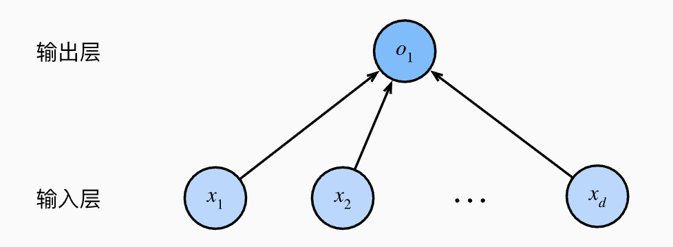
In the figure above, the input layer has \(d\) input variables, each representing a feature, i.e., the feature dimensionality is \(d\). The circle \(o_1\) represents a linear neuron, corresponding to the predicted output.
The structure shown above is also called a Fully Connected Layer (FC), also known as a Dense Layer, and is one of the most fundamental layer structures in deep learning and artificial neural networks. Its defining characteristic is: every neuron in the layer is connected to all neurons in the previous layer.
Inside a linear neuron, it performs only two operations:
- Weighted summation: multiply all inputs \(x_i\) by their corresponding weights \(w_i\) and sum them up.
- Add bias: add \(b\) at the end.
We can think of the connections in the figure as weights, representing the synaptic strength between input features and the neuron, determining how much each input signal contributes to the final result. Inside the linear neuron, a bias \(b\) is stored, which is typically viewed as an intrinsic property of the neuron \(o_1\) itself.
In other words, training a linear regression model amounts to adjusting the connection weights and bias of this linear neuron. The linear neuron determines how the prediction (\(\hat{y}\)) is produced, while the training optimization (squared loss, gradient descent) is responsible for correcting this neuron: the gradient descent algorithm computes the derivative of the loss with respect to the neuron's parameters, then tells the neuron how to adjust its weights and bias in the reverse direction to reduce the loss.
It is called a "linear neuron" because its output is merely a linear combination of the inputs.
Single-Layer Perceptron
The essence of a classification problem is finding a decision boundary. The essence of a linear model is drawing a straight line.
Rosenblatt at Cornell University, inspired by biological neurons in the brain, invented the single-layer perceptron. The single-layer perceptron uses a step function: output 1 if \(z > 0\), otherwise output 0.
Because the single-layer perceptron uses a hard threshold, it is mathematically non-differentiable, so gradient descent cannot be used for fine-grained optimization.
Minsky, in his 1969 book, proved that the single-layer perceptron cannot solve the XOR (exclusive or) problem. This was not merely a mathematical issue — it was a disaster. It demonstrated that the AI of the time had "limited intelligence," directly triggering the first AI winter.
In the supervised learning section of the machine learning notes, we have already learned about linear regression and logistic regression. However, if we want to produce a complex classification boundary, we cannot simply stack multiple linear layers, because no matter how many linear layers are stacked, the result is still a linear transformation.
The simplest example is the XOR problem. XOR (Exclusive OR) logic is straightforward: output 0 when both inputs are the same, output 1 when they differ. We can frame it as a classification task with the following data points:
- (0, 0) \(\to\) class 0
- (1, 1) \(\to\) class 0
- (0, 1) \(\to\) class 1
- (1, 0) \(\to\) class 1
If you take a piece of paper, draw a coordinate system, and plot these four points, you will find that no matter how hard you try, you cannot draw a single straight line that separates 0 from 1. A linear model (without \(\sigma\)) can only draw straight lines. A purely linear model facing XOR can achieve at most 75% accuracy (correctly classifying only 3 out of 4 points).
It was not until the 1980s that Hinton and others revived the Multilayer Perceptron (MLP) and popularized the backpropagation algorithm. It was then that people realized that chaining multiple perceptrons together into a "Multilayer Perceptron (MLP)" and replacing the hard step function with a smooth Sigmoid could truly achieve "space folding" and solve XOR.
The Sigmoid function maps \(z\) to a smooth probability between 0 and 1. Because it is smooth and differentiable, it works effectively with cross-entropy and gradient descent.
To capture nonlinear features, we need to introduce a nonlinear transformation. The most common choice is the sigmoid: \(\sigma(z) = \frac{1}{1 + e^{-z}}\). Although the sigmoid function looks simple, it accomplishes two remarkable things:
- It introduces the concepts of "threshold" and "activation": a linear function responds to every input proportionally, but sigmoid barely responds below or above a certain threshold; it reacts sharply only near 0. It behaves like a switch.
- Space warping: through this nonlinear transformation, points that were linearly inseparable in the original coordinate system (such as the four XOR points) become neatly separable by a single cut in the "folded" new space.
Applied to the XOR problem, we can decompose the solution as follows: two "steps" cooperating and folding. Suppose we have two neurons \(h_1\) and \(h_2\), each equipped with a Sigmoid.
- Neuron \(h_1\)*: it monitors *\(x_1 + x_2\). It begins to activate when either input is 1.
- Neuron \(h_2\)*: it also monitors *\(x_1 + x_2\), but it is more "sluggish" — it activates strongly only when both inputs are 1.
At this point, a space warping occurs: we map the original \((x_1, x_2)\) coordinates to the new hidden-layer axes \((h_1, h_2)\):
- For A (0,0): both neurons stay inactive \(\to\) new coordinates (0, 0)
- For C (0,1) and D (1,0): \(h_1\) activates, \(h_2\) does not \(\to\) new coordinates (1, 0)
- For B (1,1): both \(h_1\) and \(h_2\) activate \(\to\) new coordinates (1, 1)
Now, visualize the new coordinate system \((h_1, h_2)\) and plot these three new positions:
- Red points: (0, 0) and (1, 1)
- Blue points: (1, 0) (the original two blue points have merged)
These three points now form a triangle:
- The base goes from (0,0) to (1,0)
- The side goes from (1,0) to (1,1)
In the original space, red points A and B were separated by the blue points, facing each other from afar. But after the Sigmoid's nonlinear compression:
- The two blue points are "pinched" to the same position (1, 0).
- Because \(h_2\) is nonlinear (it does not rise smoothly but acts like a step), it "pulls up" the point (1,1) while keeping (1,0) low.
"The essence of solving XOR is 'feature space transformation.' Each neuron with a Sigmoid cuts through the original space and produces a nonlinear activation wave. When multiple neurons are combined, it is equivalent to performing a nonlinear bending and projection of the original flat coordinate system. In this 'crumpled' new space, originally linearly inseparable data points are rearranged so that they become linearly separable in the new dimensions. This is the fundamental logic by which neural networks solve complex problems through adding hidden layers."
In neural network terminology, the combination of a "linear operation (\(wX+b\)) + nonlinear activation function (\(\sigma\))" is called a nonlinear neuron.
The mathematical expression for a typical nonlinear neuron (with a single output) is:
In PyTorch's internals (e.g., nn.Linear paired with an activation function), the formula is usually expressed in matrix form to handle batches of data:
With the sigmoid function, all the essential elements for deep neural networks are now in place.
Softmax Regression
So far, we have covered linear regression, linear neurons, and nonlinear neurons. Now we introduce a special, "globally aware" nonlinear activation function that typically serves as the final processing step for a group of neurons, collectively transforming them into a nonlinear neural unit array.
In classification problems, if there are only two classes, we can use 1 output neuron + Sigmoid. If there are multiple output neurons and the output categories are non-mutually exclusive (e.g., an image contains both "mountain" and "water"), each neuron independently determines whether that label is present, so we can still use N output neurons + Sigmoid.
However, for multi-class classification where categories are mutually exclusive (e.g., recognizing cat, dog, or pig), the model must produce a probability distribution over these options and select the one with the highest probability. In this case, the Sigmoid function is no longer appropriate.
In deep learning, a logit typically refers to the raw numerical output of the last fully connected layer of a neural network — the result before entering an activation function (such as Softmax or Sigmoid).
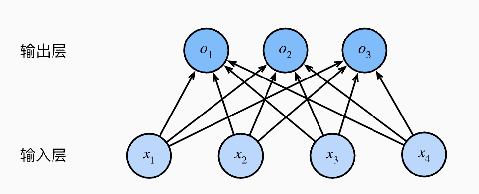
To compute the raw score (i.e., the logit) for each class, we configure an independent set of weights and biases for each output:
The three values \(o_1, o_2, o_3\) computed for each input are called "unnormalized predictions (logits)." This is essentially an affine function — a linear combination plus bias.
For efficiency in both programming and mathematical derivation, this is typically written as a matrix multiplication:
where:
- \(\mathbf{o}\): output vector, with dimensions \(3 \times 1\).
- \(\mathbf{W}\): weight matrix, with dimensions \(3 \times 4\) (corresponding to 12 scalar weights).
- \(\mathbf{x}\): input feature vector, with dimensions \(4 \times 1\).
- \(\mathbf{b}\): bias vector, with dimensions \(3 \times 1\).
In the example shown in the figure, the parameter count can be calculated as:
That is, 4 x 3 + 3 = 15 parameters. Text generation tasks like GPT are essentially giant multi-class selection machines, and the total parameter count we commonly refer to is computed by summing up parameters in exactly this manner.
Let us now examine the Softmax function itself:
From a prediction standpoint, we cannot directly treat the raw outputs (logits) of a neural network as probabilities. We want to predict the class with the highest probability, i.e., \(\operatorname{argmax}_j \hat{y}_j\) — simply put, we pick whichever class has the highest score. However, the raw values output by the last layer of the network (denoted \(o\)) cannot be called "probabilities" directly because they violate two fundamental axioms of probability: non-negativity and normalization.
Non-negativity means that a neural network's raw outputs can be negative, but probabilities must be \(\ge 0\). Normalization means that the raw outputs do not necessarily sum to \(1\), but the probabilities of all possible classes must sum to \(1\). Because the exponential function is monotonically increasing, if \(o_1 > o_2\), then \(\exp(o_1) > \exp(o_2)\). Therefore, Softmax does not change the relative ordering of the original predictions, that is:
This means that looking at the maximum of the raw outputs and looking at the maximum after Softmax yields the same result.
For the case of \(n\) samples, we can stack \(n\) samples together into a matrix and compute all predictions simultaneously via a single matrix multiplication. For example, given:
- Feature matrix \(\mathbf{X}\)*: shape *\(n \times d\), where \(n\) is the batch size (how many samples are processed at once) and \(d\) is the number of features per sample.
- Weight matrix \(\mathbf{W}\)*: shape *\(d \times q\), where \(q\) is the number of output classes (e.g., for a 10-class problem, \(q\) is 10).
- Bias vector \(\mathbf{b}\)*: shape *\(1 \times q\).
We obtain:
The matrix multiplication \(\mathbf{X}\mathbf{W}\)* yields an *\(n \times q\) matrix. Note that \(\mathbf{b}\) has only one row, while \(\mathbf{X}\mathbf{W}\) has \(n\) rows. During computation, the system automatically replicates \(\mathbf{b}\) across every row for element-wise addition — this is the highly practical broadcasting mechanism in deep learning.
Applying Softmax to each row of the result matrix \(\mathbf{O}\) converts it into a probability distribution (each row sums to 1). The resulting \(\hat{\mathbf{Y}}\) is a matrix containing the predicted probabilities for all \(n\) samples.
Cross-Entropy Loss Function
Everything discussed above can be viewed as a single-layer neural network: input data passes through a fully connected layer into the neuron layer, predictions are computed using weights and biases, and Softmax can be applied for multi-class normalization. However, obtaining predictions is not the main point of neural networks. Our goal is to obtain a set of parameters (weights and biases) that can be used for prediction, and we cannot obtain these parameters directly — they must be learned through training.
To train the model, we need a way to measure how well the prediction \(\hat{y}\) matches the true value \(y\).
Assuming the entire dataset is independently and identically distributed (i.i.d.), by maximum likelihood estimation (MLE), we want to maximize the probability of observing all true labels:
Since computing gradients of products is very difficult, we take the logarithm to convert the "product" into a "sum," and negate it to convert a "maximization problem" into a "minimization problem" — i.e., minimizing the negative log-likelihood (NLL):
This gives us the cross-entropy loss function. For any label \(\mathbf{y}\) (one-hot encoded) and predicted probability \(\hat{\mathbf{y}}\), the specific loss function is:
Note: In classification, since \(y_j\) is 1 at exactly one position and 0 elsewhere, the formula effectively simplifies to \(L = -\log \hat{y}_{\text{correct\_class}}\).
Because \(y\) is one-hot encoded (only one position is 1, the rest are 0), this formula actually only cares about the predicted probability of the correct class. The more confident you are about the correct class (\(\hat{y}_j\) closer to 1), the closer the loss is to 0.
Next, substituting the Softmax definition into the cross-entropy loss, we can obtain the derivative of the loss function with respect to the unnormalized predictions (logits) \(o_j\):
This yields the gradient formula (the most crucial result):
This derivative (gradient) is precisely the difference between the model's predicted probability and the actual observation. This remarkably simple form (predicted value - true value) makes gradient computation very easy and efficient in practice.
For a neural network, the process of passing input data through the network to produce output is called forward propagation. Next, we compare the predictions with the true values — as introduced in the machine learning notes, this involves using a loss function to quantify the discrepancy. Finally, based on the loss, we compute derivatives and update parameters in the direction of gradient descent so that the parameters move toward our target — the differentiation and chain rule portion is called backpropagation, and the parameter update portion is called optimization.
It is important to note that in vectorized computation, we typically compute the average loss over a minibatch of \(n\) samples:
This is because if the gradient magnitude fluctuates drastically with the batch size, optimization becomes unstable.
In practice, directly computing \(\exp(o_k)\) can easily cause numerical overflow. Therefore, mature deep learning frameworks (such as PyTorch) typically combine Softmax and Cross-Entropy into a single function, using the LogSumExp trick to ensure numerical stability.
It is worth noting that although cross-entropy is the loss function used during training, it is not very intuitive. During evaluation, we use accuracy instead.
where:
- \(\hat{y}_i = \operatorname{argmax}_j Q(y_{ij})\): the class with the highest predicted probability.
- \(\mathbb{1}(\cdot)\) is the indicator function, which equals 1 if the condition holds and 0 otherwise.
From an information-theoretic perspective, we can summarize as follows:
| Concept | Formula (brief) | Intuitive meaning |
|---|---|---|
| Information | \(-\log P(x)\) | The "surprise" carried by a single event |
| Entropy | \(\sum P \log \frac{1}{P}\) | The average uncertainty of the entire system |
| Cross-Entropy | \(\sum P \log \frac{1}{Q}\) | The cost of representing the true distribution \(P\) using the predicted distribution \(Q\) |
| Accuracy | Correct / Total | The model's performance in actual decision-making |
For details, see the information theory notes.
Multi-Layer Neural Networks
Above, we have learned about single-layer neural networks and understood how forward propagation works (input data passes through a fully connected layer with weights and neuron biases to produce predictions), how to evaluate predictions (for classification tasks, typically using cross-entropy loss), and how to update parameters based on the results (gradient descent, backpropagation, and parameter updates).
We have also learned about activation functions and nonlinear neurons. Next, we will design multi-layer neural networks.
Universal Approximation Theorem
In 1989, Cybenko and others formally published a paper proving mathematically that, given sufficiently many neurons with nonlinear activation functions, we can approximate any continuous function in the world. This is the Universal Approximation Theorem.
Having established the universal nature of stacking, artificial intelligence was mathematically proven capable of simulating arbitrarily complex curves through a sufficient number of nonlinear activation units. From a mathematical perspective, no matter how vast the parameter space, there must exist a set of parameters \((w, b)\) that perfectly simulates that complex curve.
Even in the Transformer-based large model era of the 2020s, the underlying mathematical principle remains the same: drawing countless extremely complex "decision boundaries" in an enormously high-dimensional space. The process by which GPT generates the next token is essentially full-vocabulary classification (choosing 1 word out of, say, 50,000). Transformers map each input token into a 12,288-dimensional vector (using GPT-3 as an example). Before the final output layer (Linear + Softmax), the model has already sorted out the "logic." At that point, the space contains 50,000 regions, each corresponding to a word. All of the Transformer's computations (Self-Attention) serve to continuously move this vector's position in the space until it lands in the "decision region" representing the correct answer. Going further, Transformers dynamically adjust the way the space is folded based on input context (e.g., whether "Apple" is followed by "company" or "phone"). This "attention mechanism" allows the model to perform a "global rearrangement" of the space at every layer, thereby carving out exquisitely precise decision boundaries in an extremely high-dimensional space.
In summary, the Universal Approximation Theorem proves that given a single hidden layer with sufficiently many neurons and nonlinear activation functions, it can approximate any continuous function on a closed interval to arbitrary precision.
Feature Hierarchy
Although the Universal Approximation Theorem (1989) established the theoretical lower bound showing the feasibility of a single layer with infinitely many neurons, virtually all neural network architectures in practice are multi-layered. In fact, scientists were already experimenting with multi-layer structures before the Universal Approximation Theorem appeared.
In 1965, Soviet mathematicians Ivakhnenko and Lapa proposed the "Group Method of Data Handling" (GMDH), which is considered the world's first true deep learning algorithm. They used multi-layer polynomial neurons to fit data, with each layer attempting to select the best features to pass to the next layer.
In 1980, Japanese scientist Kunihiko Fukushima proposed the Neocognitron. Inspired by biological vision, he designed an architecture alternating between convolutional and pooling layers. This directly influenced the later development of Convolutional Neural Networks (CNNs).
In 1986, Geoffrey Hinton, one of the three pioneers of deep learning, and his colleagues re-popularized the backpropagation algorithm. This was a historic turning point because it solved the problem of "how to train multi-layer networks."
The historical record shows that the use of multiple layers originated from biological intuition.
In the 1950s, Hubel and Wiesel's physiological experiments discovered that the cat's visual cortex is hierarchical: some cells respond only to lines, some to shapes, and some to complex objects. Deep neural networks mimic this compositional logic: complex systems are inherently hierarchical. Through multi-layer stacking, the network can first learn "local features" and then learn "global structures." This evolution from local to global is logically very difficult for a single-layer network (even a nonlinear one) to achieve.
Another hypothesis concerns "spatial transformation." The Manifold Hypothesis posits that real-world high-dimensional data (such as images and audio) actually lie on low-dimensional manifolds. In plain terms, the data is like a two-dimensional sheet of paper crumpled up in three-dimensional space. This process of "unfolding layer by layer" is called disentanglement. The significance of multiple layers is that a single transformation can rarely straighten out extremely complex distortions in one go — it takes multiple layers of continuous, smooth mappings to transform a complex manifold into a linearly separable state.
Vanishing Gradient Problem
Although scientists' biological intuition led them to experiment with multi-layer neural networks, a "signal loss" phenomenon emerged during training: when the network becomes too deep, neurons at the bottom (those closest to the input layer) fail to receive effective "correction signals," causing them to stop learning.
In neural networks, we use backpropagation to update parameters. According to the chain rule, the gradient of a deep neuron is the product of the gradients from all preceding layers.
Early neural networks commonly used the Sigmoid activation function. Its maximum derivative is only 0.25 (when the input is 0).
- If your network has 20 layers, the gradient reaching the front must be multiplied by 20 numbers less than 0.25.
- \(0.25^{20}\) is a vanishingly small number, practically zero.
Moreover, if the weights \(W\) at each layer are initialized very small, the compounding effect quickly drives the gradient to zero. The vanishing gradient problem causes the layers near the output to learn well, while the bottom layers (near the input) barely change. This means the network cannot extract basic features, and the advantages of a deep architecture are completely lost.
To address the vanishing gradient problem, several solutions have been proposed over time:
- Layer-wise pre-training
- ReLU (Rectified Linear Unit)
- Improved weight initialization (Xavier & He Initialization)
- Batch Normalization
- Residual connections (ResNet / Residual Learning)
Before 2006, deep learning was in a "winter" because people had discovered that training neural networks deeper than 3 layers with random initialization typically performed worse than a simple SVM. In 2006, Hinton proposed "Greedy Layer-wise Pre-training of Deep Belief Networks (DBN)." Hinton argued that deep networks were hard to train because the initial position was too poor. In the bottomless parameter space, random initialization is like being blindfolded and dropped into the Himalayas — you simply cannot find the deep valley called "global optimum."
Hinton's work fundamentally rewrote the fate of AI from philosophical, confidence, and technical perspectives. Before 2006, the mainstream academic community (including proponents of Support Vector Machines) believed that stacking neural networks deeper was useless and only led to intractable nonlinear chaos. However, Hinton demonstrated through experimental data to the world that, as long as training succeeds, deep architectures have a far higher ceiling than shallow ones for handling complex patterns (such as handwritten digit recognition). This directly ushered in the era of the term "Deep Learning."
Additionally, previous computer vision required experts to manually design features (e.g., defining circles and edges). Layer-wise pre-training demonstrated a possibility: models can learn the feature hierarchy by observing data on their own. Although it was unsupervised, it proved that machines can automatically construct a staircase from "pixels" to "concepts."
In 2010, in the paper "Rectified Linear Units Improve Restricted Boltzmann Machines," Nair and Hinton first introduced ReLU in Restricted Boltzmann Machines (RBMs). At the time, Hinton was still refining his pre-training theory. He found that compared to traditional Sigmoid, this "half-zero, half-linear" function better simulates the activation characteristics of biological neurons. Experimental results showed that ReLU not only sped up training but also solved some long-standing coordinate shift issues.
In 2011, Yoshua Bengio, another of the three pioneers of deep learning, and his student Xavier Glorot published "Deep Sparse Rectifier Neural Networks." They provided in-depth mathematical and biological arguments for why ReLU works well. They pointed out that the sparsity brought by ReLU — where most neurons are in an off state — makes the network more brain-like and effectively mitigates the vanishing gradient problem.
In 2012, AlexNet adopted the ReLU activation function in the ImageNet competition. Alex later presented a striking comparison in his paper: on the same task, reaching the same error rate, a network using ReLU was 6 times faster than one using Tanh! Moreover, AlexNet used an 8-layer architecture (astonishingly deep at the time) and crushed all traditional shallow algorithms by a decisive margin. At that moment, industry and academia reached a consensus: depth is more effective than width at capturing complex spatial features.
In 2015, the Microsoft Research Asia (MSRA) team led by Kaiming He proposed residual connections — one of the most important breakthroughs in the history of deep learning. Before this, networks with more than 20 layers were already very difficult to train; after ResNet, humans successfully trained 152-layer (and even 1000+ layer) neural networks for the first time. The key innovation was using simple "identity mappings" to allow gradients to flow through the network without loss.
With the rise of deep learning, mathematicians around 2017 (such as Hanin et al.) proved a "depth version" of the Universal Approximation Theorem: even when the number of neurons per layer is finite (or even fixed, as long as it is slightly larger than the input dimension), as long as the number of layers (depth) can grow without bound, the network can still approximate any function to arbitrary precision.
ReLU Activation Function
At this point, we have covered the origins and development of multi-layer structures from both historical and theoretical perspectives. Now let us study the design of multi-layer architectures.
Regardless of how many layers a neural network has, we divide it into three parts:
- Input layer
- Hidden layer(s)
- Output layer
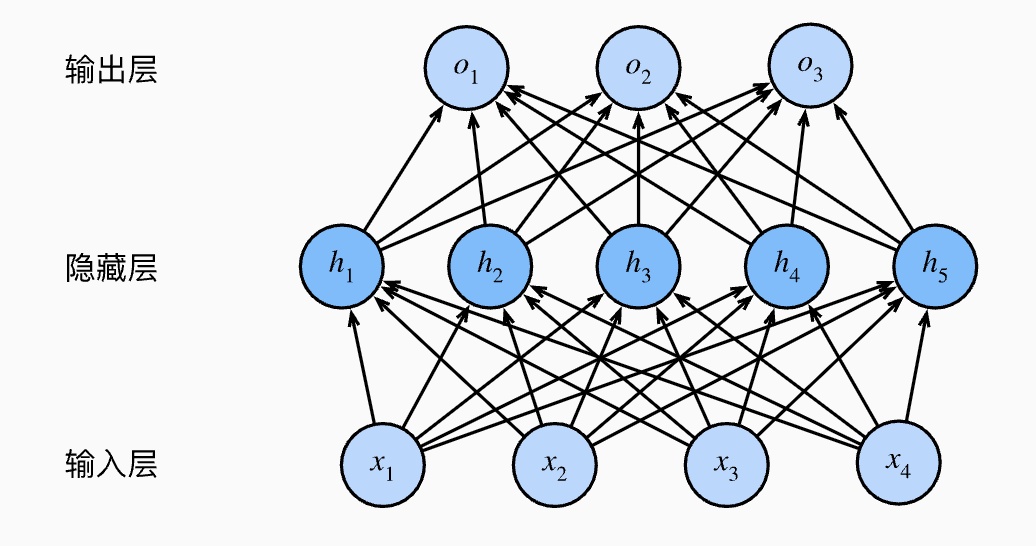
The figure above shows a multilayer perceptron with a single hidden layer containing five hidden units.
The term "hidden" is used because during training and prediction, you can only observe the inputs and outputs — the intermediate computation results (feature representations) in the middle layers are an invisible "black box" to external users.
If we use linear functions, no matter how many layers we stack, they can always be collapsed into a single layer because they are all linear transformations. Therefore, we introduce activation functions — a point that has been made repeatedly and needs no further elaboration.
We have already introduced the Sigmoid activation function and discussed its drawback in the vanishing gradient section: because both tails are nearly flat, it tends to cause vanishing gradients.
Besides Sigmoid, another common early activation function is the tanh function:
However, as mentioned in the previous subsection, the activation function that ultimately propelled deep learning to fame in 2012 was ReLU. It is fair to say that ReLU is the standard activation function of modern deep learning.
ReLU stands for Rectified Linear Unit, and its mathematical formula is disarmingly simple:
- If the input \(x > 0\): output \(x\) directly, without any modification.
- If the input \(x \le 0\): output \(0\), completely killing the signal.
Before ReLU became widespread, everyone was using Sigmoid or Tanh. ReLU solved three major pain points:
- It completely eliminates the vanishing gradient (in the positive region) — as long as \(x > 0\), its derivative is always 1. This means that whether the network has 10 or 100 layers, the gradient can flow back through the positive region "undiminished."
- The computer only needs to check
if (x > 0). This extreme simplicity dramatically reduces the cost of training large networks. - ReLU turns all negative signals to 0. This means that at any given moment, only a fraction of neurons are active while the majority are "sleeping." This closely mirrors how the biological brain works — when we think, not all neurons are firing simultaneously. This sparsity gives the model better generalization ability and makes it less prone to overfitting.
The activation function is the soul of a neural network. Without activation functions, there would be no multi-layer structures.
Of course, ReLU has a fatal flaw: if a neuron's weights are updated too aggressively, causing its input \(x\) to be negative for all training data, then:
- This neuron's output is always 0.
- Its gradient is also always 0.
- It can never be updated again, becoming a "dead" neuron.
To address the "Dead ReLU" problem, researchers have invented several variants:
- Leaky ReLU: gives the negative region a small slope (e.g., \(0.01x\)) to prevent it from dying completely.
- PReLU: the slope of the negative region is learned, not fixed.
- GeLU (Gaussian Error Linear Unit): smoother around \(0\). This is currently the preferred activation function for large models like GPT and BERT.
Multi-Layer Fully Connected Neural Network
At this point, following in the footsteps of our predecessors, we have designed the Multilayer Perceptron (MLP). In simple terms, an MLP is a neural network composed of several fully connected layers. A multi-layer fully connected neural network is also called an MLP, FCNN, or FNN.
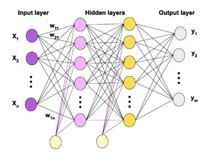
We can observe the following characteristics of this type of neural network:
- Signals always flow from the input layer, through the hidden layers, and finally to the output layer. This is why it is also called a feedforward neural network.
- Fully connected: every neuron in layer \(n\) is connected to all neurons in layer \(n-1\).
- The connections between any two adjacent layers can be represented by a large weight matrix \(W\).
- The output of each layer is \(Output = \sigma(W \cdot Input + b)\), where \(\sigma\) is the activation function.
A brief note on ResNet: as mentioned earlier, the introduction of residual connections opened the door to the era of deep architectures. The principle behind ResNet is remarkably simple:
- Standard feedforward layer: \(y = f(x)\)
- Residual feedforward layer: \(y = f(x) + x\)
Since ResNet is predominantly applied in CNNs, I will discuss ResNet in detail in the CNN notes.
The Learning Process of Neural Networks
The entire learning process is also known as optimization. For detailed content, see the optimization notes — this section provides only a preliminary overview. It is called optimization because, in mathematics and engineering, it is a standard optimization problem.
Initialization
Before learning begins, we need to assign initial values to all parameters (weights \(W\) and biases \(b\)) in the network. We typically cannot set them all to 0 (otherwise neurons will suffer from symmetry issues); instead, we use random initialization (e.g., from a Gaussian distribution) or specialized methods (such as Xavier or He initialization).
- He initialization (commonly used): \(W \sim N(0, \frac{2}{n_{in}})\)
The purpose is to prevent signal vanishing or exploding in deep networks.
Forward Propagation
Data enters at the input layer and flows forward layer by layer.
- Linear computation: each layer computes \(z = Wx + b\).
- Nonlinear activation: an activation function (such as ReLU or Sigmoid) produces the output.
- Obtain result: the final layer outputs a prediction \(\hat{y}\).
Each layer essentially does two things: linear transformation + nonlinear activation.
- Linear weighted sum: \(z^{(l)} = W^{(l)} a^{(l-1)} + b^{(l)}\)
- Activation: \(a^{(l)} = \sigma(z^{(l)})\)
- (\(\sigma\) is the activation function, e.g., ReLU: \(\max(0, z)\))
Loss Computation
We compare the prediction \(\hat{y}\) with the true label \(y\), using a loss function to measure how poorly the model predicts — quantifying the "error" as a concrete number.
Common functions: Mean Squared Error (MSE) for regression, Cross-Entropy for classification.
- Mean Squared Error (MSE, for regression): \(L = \frac{1}{2} \|y - \hat{y}\|^2\)
- Cross-Entropy (for classification): \(L = -\sum y \log(\hat{y})\)
Backpropagation
This is the most critical step, and its purpose is to compute the gradients.
- Chain rule: starting from the output layer, the chain rule from calculus is used to compute the partial derivative (gradient) of the loss function with respect to every parameter in every layer.
- Assigning responsibility: the gradient tells us how much the total error would change if a given weight were adjusted slightly.
The core of this step is the chain rule — computing the partial derivatives (gradients) of the loss \(L\) with respect to the parameters.
-
Output layer error:
$$ \delta^{(L)} = \frac{\partial L}{\partial a^{(L)}} \cdot \sigma'(z^{(L)}) $$
(i.e., derivative of the loss w.r.t. the output \(\times\) derivative of the activation function) 2. Layer-by-layer gradient propagation:
$$ \delta^{(l)} = ((W^{(l+1)})^T \delta^{(l+1)}) \cdot \sigma'(z^{(l)}) $$
(This step embodies the "backward" nature: the error at layer \(l\) is derived from the error at layer \(l+1\)) 3. Final parameter gradients:
$$ \frac{\partial L}{\partial W^{(l)}} = \delta^{(l)} (a^{(l-1)})^T, \quad \frac{\partial L}{\partial b^{(l)}} = \delta^{(l)} $$
.
Parameter Update
Using the computed gradients, we take a small step in the direction that reduces the error.
-
Stochastic Gradient Descent (SGD):
\[ W_{new} = W_{old} - \eta \cdot \frac{\partial L}{\partial W} \](\(\eta\) is the learning rate, which determines how large a step to take)
.