FGSM & PGD
FGSM (Fast Gradient Sign Method) and PGD (Projected Gradient Descent) are both gradient-based white-box attack methods. Because they share the same theoretical foundation, we cover them together in this chapter. FGSM is the pioneering method, while PGD is its most widely used and strengthened variant.
The timeline of FGSM and PGD family attack algorithms is as follows:
| Year | Algorithm | Key Paper | Key Milestone / Contribution |
|---|---|---|---|
| 2013.12 | L-BFGS | Intriguing properties of neural networks | Foundational work. First discovery of adversarial examples; used a second-order optimization algorithm to find perturbations. |
| 2014.12 | FGSM | Explaining and Harnessing Adversarial Examples | Efficiency revolution. Goodfellow proposed the linear hypothesis, reducing the attack to a single-step gradient computation and drastically lowering computational cost. |
| 2015.11 | DeepFool | DeepFool: a simple and accurate method to fool deep neural networks | Precision improvement. Iteratively pushes samples toward the nearest decision boundary, producing perturbations smaller and less perceptible than FGSM. |
| 2016.07 | BIM / I-FGSM | Adversarial examples in the physical world | Iterative refinement. First decomposed FGSM into multiple small steps, and demonstrated that adversarial examples remain effective in the physical world (e.g., printed and re-photographed). |
| 2016.08 | C&W Attack | Towards Evaluating the Robustness of Neural Networks | Breaking defenses. Designed to defeat the then-popular "distillation defense," it formulates the attack as a highly refined optimization problem and serves as the "gold standard" for evaluating model robustness. |
| 2017.06 | PGD | Towards Deep Learning Models Resistant to Adversarial Attacks | Strongest attack / defense foundation. Introduced random initialization and projection, proving PGD to be the "optimal first-order attack" under \(L_\infty\) constraints, and the cornerstone of adversarial training. |
| 2017.10 | MIM | Boosting Adversarial Attacks with Momentum | Improved transferability. Incorporated momentum into the iterative process, addressing the tendency of iterative attacks to get stuck in local optima, and significantly boosting black-box attack success rates. |
.
Mathematical Foundations
Core Idea
During model training, our goal is to find the optimal parameters \(\theta\) that minimize the gap between predictions and the ground-truth labels \(y\). We fix the input \(x\), adjust the parameters \(\theta\), and update \(\theta\) via gradient descent along the negative gradient direction. In other words, we reduce the loss to push model predictions closer to the correct label \(y\):
In adversarial attacks, however, we assume the model is already trained. We fix \(\theta\) and instead modify the input \(x\). Our goal is to find a small perturbation \(\Delta x\) that maximizes the loss function — that is, to push the model's prediction away from the correct label \(y\):
This is the fundamental idea behind adversarial attacks.
In adversarial attacks, there are two key variables:
- Minimizing the perturbation \(\Delta x\) — keeping it imperceptible to the human eye for stealth.
- Maximizing the loss — ensuring the model misclassifies.
Mathematically, this is a constrained optimization problem. We typically fix one objective and optimize the other.
As we know, neural networks are highly complex. Goodfellow proposed a remarkable insight: in extremely high-dimensional spaces, activation functions like ReLU and Sigmoid, along with the multi-layer architecture, behave not as highly twisted nonlinear mappings, but rather as approximately linear, "straightened-out" functions.
This perspective is not meant for rigorous mathematical proof but for practical use. If we tried to account for every curve and bend, the computational cost would explode. Goodfellow argued that although the model is globally nonlinear, within the tiny neighborhood of an adversarial perturbation, nonlinearity (curvature) is not the primary cause of failure — linearity (slope) is. As long as the model has even a slight slope locally, that slope gets amplified enormously in high-dimensional space.
Under this assumption, we use a Taylor expansion to approximate the complex function with a simple polynomial. This is analogous to standing on a hillside: although we cannot see the distant terrain, we know the small patch under our feet, and we can extend it outward to treat the slope as a flat, tilted plane:
- Zero-order approximation: \(L(x + \eta) \approx L(x)\) (assume perfectly flat, no change in height).
- First-order approximation (linear approximation): \(L(x + \eta) \approx L(x) + \text{slope} \times \text{distance}\).
Here, the slope is the gradient \(\nabla_x L\). So the formula:
essentially says: new height \(\approx\) old height + (slope \(\times\) step taken). The last term \(\nabla_x L^T \cdot \eta\) is the dot product of two vectors. By linear algebra, the dot product of two vectors \(\vec{A}\) and \(\vec{B}\) is:
where \(\theta\) is the angle between the two vectors. We want to maximize this value. Since \(\|\vec{A}\|\) (the gradient magnitude) and \(\|\vec{B}\|\) (the perturbation magnitude) are relatively fixed, the only variable is \(\cos(\theta)\). Therefore, when \(\theta = 0^\circ\) (i.e., the two vectors point in exactly the same direction), \(\cos(0^\circ) = 1\), and the dot product is maximized.
The above explains why we add perturbation along the gradient direction — it is logically the direction that increases the loss function the fastest.
In summary, all gradient-based attacks follow the core assumptions and concepts outlined above:
- Same objective: \(\max_{\Delta x} L(f_\theta(x + \Delta x), y)\).
- Same assumption: Local linearity assumption + first-order Taylor expansion.
- Same driving force: Maximize the dot product by aligning the perturbation direction with the gradient direction (\(\theta = 0^\circ\)).
Gradient Ascent Attack
We know that model training uses gradient descent:
Gradient ascent simply reverses the direction:
Here \(\alpha\) is the step size, and \(\nabla_x L\) is the gradient of the loss function with respect to the input \(x\).
This is the gradient ascent attack. It directly leverages the gradient of the loss with respect to the input, iteratively modifying the input image until the model's prediction is completely wrong. It is typically written as:
- \(x_t\): The image at iteration \(t\).
- \(\alpha\): Step size (learning rate), controlling how far to move each step.
- \(\nabla_{x_t} L\): The gradient computed from the current image.
In practice, gradient ascent attacks come in two flavors:
- Unconstrained attack — no limit on the size of \(\Delta x\). This kind of attack succeeds easily and can push the loss very high, but the image becomes covered in snowflake-like noise or even turns into complete visual chaos. It is immediately obvious to the human eye and thus fails the stealth requirement.
- Constrained attack (BIM) — the total perturbation is bounded. A common choice is the \(L_2\) constraint (bounding the sum of squared pixel changes).
In constrained attacks, the general procedure is:
- Compute the gradient.
- Take a small step along the gradient.
- Check: If the total perturbation exceeds the budget, scale all pixel changes back proportionally (this is the so-called "projection").
Although plain gradient ascent is less commonly used than FGSM in the image domain, it is the theoretical foundation of all iterative attacks (such as PGD).
- FGSM "simplifies" gradient ascent into a single-step sign operation.
- PGD "refines" gradient ascent — it is essentially constrained multi-step gradient ascent.
FGSM
Mathematically, the dot product of two vectors \(\vec{A}\) and \(\vec{B}\), i.e., \(\vec{A}^T \cdot \vec{B}\), is the sum of their element-wise products. Let the gradient vector be \(g = \nabla_x L\). Then the objective to maximize, \(\nabla_x L^T \cdot \eta\), can be written as:
Here \(i\) indexes each pixel in the image (for example, a 224x224 image has \(i\) ranging from 1 to 50,176). Since the perturbation \(\eta_i\) for each pixel \(i\) is independent, maximizing the total sum amounts to making each individual term \(g_i \cdot \eta_i\) as large as possible.
Now consider a single pixel \(i\):
- Known quantity: \(g_i\) (the gradient computed by the model, which can be positive or negative).
- Constraint: \(|\eta_i| \le \epsilon\) (meaning \(\eta_i\) must lie in the interval \([-\epsilon, \epsilon]\)).
- Goal: Choose an \(\eta_i\) that maximizes \(g_i \cdot \eta_i\).
We consider two cases:
- If \(g_i > 0\) (positive gradient). To maximize \(g_i \cdot \eta_i\), since \(g_i\) is positive, we want \(\eta_i\) to be as large as possible. Under the \([-\epsilon, \epsilon]\) constraint, the maximum value is \(\epsilon\). Then \(g_i \cdot \eta_i = g_i \cdot \epsilon\).
- If \(g_i < 0\) (negative gradient). Note that since \(g_i\) is negative, to make the product \(g_i \cdot \eta_i\) a large positive number, \(\eta_i\) must also be negative (a negative times a negative is positive). Under the \([-\epsilon, \epsilon]\) constraint, the most negative value is \(-\epsilon\). Then \(g_i \cdot \eta_i = (-|g_i|) \cdot (-\epsilon) = |g_i| \cdot \epsilon\).
- If \(g_i = 0\). Regardless of the value of \(\eta_i\), the product is 0, contributing nothing to increasing the loss (typically ignored).
We thus discover that regardless of whether \(g_i\) is positive or negative, to achieve maximization, the absolute value of \(\eta_i\) is always \(\epsilon\), and its sign always follows \(g_i\). This is precisely the definition of the sign function \(\text{sign}(x)\):
Therefore, the optimal \(\eta_i\) can be written as:
Combining all pixels back into vector form, we obtain the core component of FGSM: \(\eta\). The Greek letter \(\eta\) (Eta) is commonly used in mathematics to denote "perturbation" or "noise":
That is:
Our goal is to add a perturbation to the original image \(x\):
This gives us the FGSM attack formula:
- \(J(\theta, x, y)\): Model loss function.
- \(\nabla_x\): Gradient with respect to input \(x\).
- \(\text{sign}(\cdot)\): Sign function (extracts only the sign).
- \(\epsilon\): Perturbation magnitude, controlling attack intensity.
.
PGD
As shown above, FGSM performs a single-step attack on the image — regardless of where that step leads, it takes only one step. We use epsilon to limit the step size, thereby controlling the perturbation strength so that the image does not change too much.
PGD extends FGSM by replacing the single step with many small steps, each of size alpha. After each step, the result is projected (clipped) back into the allowed perturbation range:
- \(\Pi_{x+S}\): Projection operator, ensuring the adversarial example always stays within an \(\epsilon\)-radius ball centered at \(x\).
- \(\alpha\): Step size.
Multiple steps are generally stronger than a single step because the multi-step process can continuously climb along the local landscape of the nonlinear model.
An important note: since FGSM performs only one update and then clips to the valid range, whereas PGD repeats for T iterations, projection must be applied at every iteration. Projection means pulling \(\delta\) back into the valid range, i.e., \(\lvert \lvert \delta \rvert \rvert _\infin \in [0,1]\), while ensuring \(x+\delta \in [0,1]\) (or the normalized range). The \(L_\infty\) norm constrains the maximum change of each individual pixel (e.g., each pixel can change by at most 8 gray levels). This is the most commonly used norm because it ensures no single location in the image looks conspicuous.
Note that PGD performs T iterative updates to the perturbation. At each iteration, it applies a small update (with step size \(\alpha\) and direction sign(\(\Delta\))) to every pixel across all channels of the entire image, then projects back. The per-step projection ensures the perturbation does not exceed \(\epsilon\) and the image values remain within the valid range.
Targeted Attack
So far, we have assumed the perturbation is untargeted — the goal is simply to make the model more likely to err, so we perturb along the gradient ascent direction. If we instead want to steer the model toward a specific target class or target text \(y_t\), we need to minimize the loss with respect to the target.
Untargeted FGSM (the default formula):
Targeted FGSM:
In the formulas above, \(y\) and \(y_t\) represent:
- \(y\), ground-truth or true label — the class the image should actually be classified as, e.g., "cat," hence \(x + ...\)
- \(y_t\), target label or target class — the class we want the model to predict, hence \(x - ...\)
The same applies to PGD. Untargeted PGD:
Targeted PGD:
.
FGSM Attack Example
Review of Principles
From an optimization perspective, our goal is to maximize the loss:
where delta is the perturbation. The constraint is \(L_{\infin}\), meaning each pixel can change by no more than epsilon. Under this constraint, we maximize the loss. The loss essentially measures "how far the model's prediction is from the true label." A larger loss means the model deviates more from the correct answer.
FGSM solution:
Final adversarial example:
.
To quantify "whether the perturbation is visible to the human eye," three norms are commonly used:
- \(L_\infty\) norm: Constrains the maximum change of each individual pixel (e.g., each pixel can change by at most 8 gray levels). This is the most commonly used norm because it guarantees no single location in the image appears conspicuous.
- \(L_2\) norm: Constrains the sum of squares of all pixel changes (total energy). It allows some pixels to change more, as long as the overall change remains small.
- \(L_0\) norm: Constrains how many pixels can be changed (e.g., only 10 pixels in the entire image may be modified, but by any amount).
It is worth noting that these norms are not specific to adversarial attacks. However, \(L_\infty\) has become the star of adversarial attacks because its strict limit on the maximum per-pixel change aligns best with the human visual system — if no single point looks conspicuous, the image as a whole appears unchanged.
Using the \(L_\infty\) (infinity norm) perturbation constraint, the FGSM formula is:
where:
- \(x\): Original input image
- \(y\): True label
- \(f(x)\): Model output logits
- \(L(\cdot)\): Loss function (typically cross-entropy)
- \(∇xL\): Gradient of the loss with respect to input x
- \(sign(\cdot)\): Gradient sign function
- \(\epsilon\): Perturbation magnitude (must be explicitly specified)
clip: Clips the generated adversarial image back to the valid input range
Note that FGSM is a single-step attack — it performs only one attack step. Mathematically, it is essentially a one-shot linear approximation:
Subject to the constraint:
The optimal solution is:
The clip in the formula means "clamp the values to the valid range." After adding the perturbation, the adversarial example may exceed the allowed input range, e.g., going beyond the pixel space [0,1] or the normalized range [-1,1]. Therefore, it needs to be clamped back:
In PyTorch, the clamp function implements clip:
adv_image = adv_image.clamp(-1, 1)
This restricts every element of adv_image to the range [-1, 1]:
- Values below -1 become -1
- Values above 1 become 1
- Values in between remain unchanged
FGSM Attack
FGSM (Fast Gradient Sign Method) is the simplest adversarial attack method, proposed by Goodfellow et al. in 2014. Its core formula is:
Breaking it down:
- \(\nabla_x L(f(x), y))\): The gradient of the loss with respect to the input image. During normal training, we compute the gradient of the loss with respect to the weights to update them. Here, we do the reverse — fix the weights and compute the gradient with respect to the input pixels, indicating "in which direction should pixels change to increase the loss the fastest."
- sign(·): Takes only the sign of the gradient (+1 or -1), discarding the magnitude. This way, each pixel is either increased or decreased by exactly ε, giving full control over the perturbation magnitude.
- ε (epsilon): Perturbation strength. Typical test values are 2/255, 4/255, 8/255. Since pixel values range from 0 to 255, 8/255 represents roughly a 3% change in pixel value — nearly imperceptible to the human eye.
- clip: Clamps the perturbed pixel values back to the valid range ([-1, 1] after normalization) to prevent values from exceeding the image's valid domain.
With these principles understood, the implementation is straightforward:
- Compute the gradient of the loss with respect to the input image.
- Add a small perturbation to the image in the gradient ascent direction.
When applying the perturbation, note that the input image in a neural network is essentially a 4D tensor:
For example, CIFAR-10 uses \((1,3,32,32)\). Each element, after normalization, is a pixel value between -1 and 1. For instance:
Its gradient is:
Taking the sign of the gradient gives -1, so the perturbation is \(\epsilon \cdot (-1)\), and the new pixel value becomes \(0.24-\epsilon\). In essence, we are simply adding or subtracting a very small number to each pixel.
Note that FGSM adds a perturbation to every single pixel in the entire image, not just a few selected points:
Furthermore, FGSM computes the gradient only once per image and generates the perturbation in a single pass.
Significance and Analysis
Three natural questions arise:
- How much change — or how large must epsilon be — to cause misclassification?
- Why can such a small perturbation be effective?
- What is the significance of this kind of perturbation?
First, although there is no fixed epsilon value, for well-studied datasets like CIFAR-10 or ImageNet, there are typical ranges:
| ε (pixel) | ε (normalized) | Human perception | Effect on model |
|---|---|---|---|
| 1/255 | 0.004 | Completely invisible | Almost no effect |
| 2/255 | 0.008 | Invisible | Minor misclassifications |
| 4/255 | 0.016 | Invisible | Significant misclassifications |
| 8/255 | 0.031 | Nearly invisible | Heavy misclassification (commonly used) |
| 16/255 | 0.062 | Slight noise | Very high error rate |
| 32/255 | 0.125 | Obvious noise | Almost entirely wrong |
Among these, 8/255 is the most commonly used standard — it is the sweet spot where the perturbation is imperceptible to the eye yet significantly degrades model accuracy.
For example:
Normal:
airplane: 0.92
bird:     0.04
cat:      0.02

After attack:
airplane: 0.12
bird:     0.18
cat:      0.51   ← misclassified
The reason such a small perturbation can fool the model is that neural networks are compositions of high-dimensional linear systems. For CIFAR-10, the image dimensionality is \(3 \times 32 \times 32 = 3072\). If each pixel changes by only 0.03, the total accumulated change can reach 100.
In other words, consider a classifier:
If each \(x_i\) increases by 0.03, the total change is:
This can be very large.
The "total change" here refers to the total impact on the model output (score/logit), not the image values themselves. The key insight is that the first layer of a neural network is essentially a weighted sum.
Gradient-based noise is the most effective attack direction. Compared to random noise, gradient noise specifically targets the model's weaknesses. In the high-dimensional space of neural network class partitions, it essentially shifts the data point's position from one side of the decision boundary to the other.
PyTorch Example
We use the CIFAR-10 dataset and a ResNet architecture to demonstrate the FGSM attack.
The necessary package imports and dataset loading are as follows:
## Your potential Task:
##Your Package imported

## For your reference, here is the package I am using

import torch
import torch.nn as nn
import torch.nn.functional as F
import torch.optim as optim
import torchvision
import torchvision.transforms as transforms
from torch.utils.data import DataLoader
import matplotlib.pyplot as plt
from IPython.display import display, clear_output
import pandas as pd
# You can also write your own data loading code
# I split the training set into training set and val set
# to use train/val only in training, without test set.
from torch.utils.data import Subset

# === 数据增强(Data Augmentation)===
# 注意:增强只能加在训练集的 transform 里,不能加在 val/test 上。
# 原因:val 和 test 需要稳定、可复现的评估结果;
#       如果对它们随机裁剪/翻转,每次评估结果都不一样,失去了参考意义。
# 因此需要为训练集和评估集定义两套不同的 transform。

# 训练集 transform:加入随机增强,人为扩充训练数据的多样性
train_transform = transforms.Compose([
    # RandomCrop: 先在图片四周各填充 4 个像素(padding=4),再随机裁剪回 32x32
    # 模拟图片平移,让模型学会识别不同位置的目标
    transforms.RandomCrop(32, padding=4),
    # RandomHorizontalFlip: 以 50% 概率随机水平翻转图片
    # 对 CIFAR-10 的大多数类别(车、鸟、船等)来说,翻转后语义不变
    transforms.RandomHorizontalFlip(),
    transforms.ToTensor(),
    transforms.Normalize((0.5, 0.5, 0.5), (0.5, 0.5, 0.5))
])

# 评估集 transform:只做必要的归一化,不做任何随机变换
eval_transform = transforms.Compose([
    transforms.ToTensor(),
    transforms.Normalize((0.5, 0.5, 0.5), (0.5, 0.5, 0.5))
])

# 加载两份原始数据集(数据文件相同,只是 transform 不同)
# full_trainset 用于探查 .classes 等属性
full_trainset     = torchvision.datasets.CIFAR10(root='./data', train=True,
                                                  download=True, transform=train_transform)
full_trainset_eval = torchvision.datasets.CIFAR10(root='./data', train=True,
                                                   download=True, transform=eval_transform)

# 用固定随机种子切分索引,保证 train/val 每次划分一致
val_size   = 5000
train_size = len(full_trainset) - val_size
generator  = torch.Generator().manual_seed(42)   # 固定种子,结果可复现
indices    = torch.randperm(len(full_trainset), generator=generator).tolist()

# train split:使用带增强的 full_trainset
# val split:使用不带增强的 full_trainset_eval(相同索引,不同 transform)
trainset = Subset(full_trainset,      indices[val_size:])
valset   = Subset(full_trainset_eval, indices[:val_size])

trainloader = DataLoader(trainset, batch_size=64, shuffle=True)
valloader   = DataLoader(valset,   batch_size=64, shuffle=False)

# 测试集:只用 eval_transform,不做增强
testset    = torchvision.datasets.CIFAR10(root='./data', train=False,
                                          download=True, transform=eval_transform)
testloader = DataLoader(testset, batch_size=64, shuffle=False)
Inspecting the dataset:
import numpy as np
import matplotlib.pyplot as plt

# full_trainset 保留了 .classes 属性,trainset/valset 是 Subset 没有该属性
classes = full_trainset.classes

# === 基本信息 ===
print(f"Full train set : {len(full_trainset)}")
print(f"  -> Train split: {len(trainset)}")
print(f"  -> Val   split: {len(valset)}")
print(f"Test set       : {len(testset)}")

# 取一张图看格式(从 full_trainset 取,Subset 索引机制不同)
sample_img, sample_label = full_trainset[0]
print(f"\nSingle image tensor shape : {sample_img.shape}")
print(f"Pixel range               : [{sample_img.min():.3f}, {sample_img.max():.3f}]")
print(f"Label example             : {sample_label} -> '{classes[sample_label]}'")

# === 查看一个 batch 的 shape ===
sample_batch_imgs, sample_batch_labels = next(iter(trainloader))
print(f"\nOne batch shape : {sample_batch_imgs.shape}")
print(f"Label shape     : {sample_batch_labels.shape}")

# === 可视化每个类别的样例图片 ===
fig, axes = plt.subplots(2, 5, figsize=(12, 5))
shown = {i: False for i in range(10)}

for img, label in full_trainset:
    label = int(label)
    if not shown[label]:
        ax = axes[label // 5][label % 5]
        npimg = (img.numpy() * 0.5 + 0.5).transpose(1, 2, 0)
        ax.imshow(np.clip(npimg, 0, 1))
        ax.set_title(classes[label])
        ax.axis('off')
        shown[label] = True
    if all(shown.values()):
        break

plt.suptitle("CIFAR-10 Sample Images (32x32)", fontsize=13)
plt.tight_layout()
plt.show()

# === 各类别样本数量分布 ===
from collections import Counter
label_counts = Counter([label for _, label in full_trainset])
print("\nFull training set class distribution:")
for i, cls in enumerate(classes):
    print(f"  {cls:>10}: {label_counts[i]}")
The model architecture is as follows:
import torch
from torch import nn

class BasicBlock(nn.Module):
    """
    ResNet 的基本构建块(Basic Block)。
    结构:Conv -> BN -> ReLU -> Conv -> BN -> (+shortcut) -> ReLU

    核心思想:残差连接(skip connection)
    让输出 H(x) = F(x) + x,模型只需学习残差 F(x) = H(x) - x。
    这样梯度可以直接通过 shortcut 回传,解决了深层网络的梯度消失问题。

    当 stride != 1 或通道数变化时,shortcut 需要用 1x1 Conv 匹配维度。
    """
    def __init__(self, in_channels, out_channels, stride=1):
        super().__init__()
        # 主路径:两个 3x3 卷积,Conv -> BN -> ReLU -> Conv -> BN
        self.conv1 = nn.Conv2d(in_channels, out_channels,
                               kernel_size=3, stride=stride, padding=1, bias=False)
        self.bn1   = nn.BatchNorm2d(out_channels)
        self.relu  = nn.ReLU(inplace=True)
        self.conv2 = nn.Conv2d(out_channels, out_channels,
                               kernel_size=3, stride=1, padding=1, bias=False)
        self.bn2   = nn.BatchNorm2d(out_channels)

        # shortcut 路径:当 stride != 1 或通道数变化时,用 1x1 Conv 对齐维度
        self.shortcut = nn.Sequential()
        if stride != 1 or in_channels != out_channels:
            self.shortcut = nn.Sequential(
                nn.Conv2d(in_channels, out_channels,
                          kernel_size=1, stride=stride, bias=False),
                nn.BatchNorm2d(out_channels)
            )

    def forward(self, x):
        out = self.relu(self.bn1(self.conv1(x)))  # Conv -> BN -> ReLU
        out = self.bn2(self.conv2(out))            # Conv -> BN
        out += self.shortcut(x)                   # 残差加法:F(x) + x
        out = self.relu(out)
        return out


class ResNet18(nn.Module):
    """
    ResNet-18 for CIFAR-10.
    结构:
      stem:    Conv3x3(3->64, stride=1) + BN + ReLU   [不降采样,保留 32x32]
      layer1:  2x BasicBlock(64->64,   stride=1)       [32x32]
      layer2:  2x BasicBlock(64->128,  stride=2)       [16x16]
      layer3:  2x BasicBlock(128->256, stride=2)       [ 8x8]
      layer4:  2x BasicBlock(256->512, stride=2)       [ 4x4]
      head:    AdaptiveAvgPool2d(1) + Flatten + Linear(512->10)
    """
    def __init__(self, num_classes=10):
        super().__init__()
        # stem: 用 3x3 conv(stride=1) 替代原版 7x7 conv(stride=2),适配 32x32 输入
        self.stem = nn.Sequential(
            nn.Conv2d(3, 64, kernel_size=3, stride=1, padding=1, bias=False),
            nn.BatchNorm2d(64),
            nn.ReLU(inplace=True)
        )
        self.layer1 = self._make_layer(64,  64,  num_blocks=2, stride=1)
        self.layer2 = self._make_layer(64,  128, num_blocks=2, stride=2)
        self.layer3 = self._make_layer(128, 256, num_blocks=2, stride=2)
        self.layer4 = self._make_layer(256, 512, num_blocks=2, stride=2)

        # 全局平均池化后 flatten,接一个全连接层输出 10 类
        self.head = nn.Sequential(
            nn.AdaptiveAvgPool2d(1),  # 任意空间尺寸 -> 1x1
            nn.Flatten(),
            nn.Linear(512, num_classes)
        )

    def _make_layer(self, in_channels, out_channels, num_blocks, stride):
        # 第一个 block 负责下采样(stride),后续 block stride=1
        layers = [BasicBlock(in_channels, out_channels, stride)]
        for _ in range(1, num_blocks):
            layers.append(BasicBlock(out_channels, out_channels, stride=1))
        return nn.Sequential(*layers)

    def forward(self, x):
        x = self.stem(x)
        x = self.layer1(x)
        x = self.layer2(x)
        x = self.layer3(x)
        x = self.layer4(x)
        x = self.head(x)
        return x


net = ResNet18(num_classes=10)
print(net)

# 验证 forward pass 维度正确
dummy = torch.zeros(1, 3, 32, 32)
print(f"\nOutput shape: {net(dummy).shape}")  # 应为 torch.Size([1, 10])
Training the model and saving checkpoints:
device = torch.device("cuda:0" if torch.cuda.is_available() else "cpu")
## Code Starting Here
# The training code references the training code I used in CS130 and CS137.

# 首先将数据集分成若干份,其数量=总数据集数量/批次大小.
# 我们设置了batch_size = 64,这个的意思就是每次喂给模型64张图片。
# iterations = len(trainset) / 64 = 781
# 这个长度的意思是每一个epoch我们要跑781个batch,才能把整个数据集跑完
# 一次iteration,就是跑完了一个batch,也就是看了64张图片。
# 一次epoch,就是跑完了所有的图片,也就是跑完781次iteration。

model = net.to(device)

criterion = nn.CrossEntropyLoss()

# 优化器:SGD + Momentum + Weight Decay(ResNet 原论文配置,泛化性优于 AdamW)
# - lr=0.1:SGD 的初始学习率通常比 Adam 大得多
# - momentum=0.9:动量,让梯度更新方向带有"惯性",有助于冲出局部最优、加速收敛
# - weight_decay=5e-4:L2 正则化系数,让权重保持小值,防止过拟合
optimizer = torch.optim.SGD(model.parameters(),
                            lr=0.1,
                            momentum=0.9,
                            weight_decay=5e-4)

# 学习率调度器:MultiStepLR
# 在指定的 epoch 到达时,将学习率乘以 gamma(即缩小为原来的 1/10)
# 训练前期用大 lr 快速下降,后期用小 lr 精细收敛:
#   epoch  1-59: lr = 0.1
#   epoch 60-79: lr = 0.01
#   epoch 80+:   lr = 0.001
scheduler = torch.optim.lr_scheduler.MultiStepLR(optimizer, milestones=[60, 80], gamma=0.1)

import os
os.makedirs('./resnet_checkpoints', exist_ok=True)

train_losses = []
test_accuracies = []
best_acc = 0.0

# 100 epoch:配合 MultiStepLR 在第 60、80 轮衰减学习率
num_epochs = 100
for epoch in range(num_epochs):
    # 使用nn.Module类,切换.train()开关
    # 这里的.train()是开关,主要是dropout和batchNorm这种特殊层在训练和测试时动作不一样
    # dropout:评估时不随机关闭神经元
    # BatchNorm,停止计算,这个后面再说,这里暂时不问
    model.train()

    # running loss是用来手动记录训练误差的变量
    running_loss = 0.0

    # for image, label in trainloader:
    for images, labels in trainloader:
        images, labels = images.to(device), labels.to(device)

        # 清除上一个batch留下的梯度,因为PyTorch默认梯度是累积的。
        optimizer.zero_grad()

        # 前向传播,得到预测结果
        outputs = model(images)

        # 对比预测结果和实际结果,算出loss(交叉熵损失函数)
        loss = criterion(outputs, labels)

        # 反向传播,算出每一层的梯度。
        loss.backward()

        # 更新参数
        optimizer.step()

        # 在PyTorch中,loss是一个带有计算图的tensor,直接累加是不合适的
        # .item()可以把tsnor中具体的数字抠出来,变成轻量级的python浮点数
        running_loss += loss.item()

    avg_loss = running_loss / len(trainloader)
    train_losses.append(avg_loss)

    # 在验证集上评估(val set 从训练集切出,用于训练过程监控)
    model.eval()
    correct = 0
    total = 0
    with torch.no_grad():
        for images, labels in valloader:
            images, labels = images.to(device), labels.to(device)
            outputs = model(images)
            _, predicted = torch.max(outputs, 1)
            total += labels.size(0)
            correct += (predicted == labels).sum().item()

    val_acc = 100 * correct / total
    test_accuracies.append(val_acc)

    # scheduler.step() 必须在每个 epoch 结束后调用,触发学习率按计划衰减
    scheduler.step()
    current_lr = scheduler.get_last_lr()[0]

    print(f"Epoch [{epoch+1}/{num_epochs}]  Loss: {avg_loss:.4f}  Val Acc: {val_acc:.2f}%  LR: {current_lr:.5f}")

    # 每次验证集准确率创新高时,覆盖保存 best_model(用于部署)
    if val_acc > best_acc:
        best_acc = val_acc
        torch.save(model.state_dict(), './best_model_resnet.pth')
        print(f"  -> New best val accuracy: {best_acc:.2f}%, best model saved.")

    # 每5轮保存一次checkpoint(包含 scheduler 状态,方便从中断处恢复训练)
    if (epoch + 1) % 5 == 0:
        torch.save({
            'epoch': epoch + 1,
            'model_state_dict': model.state_dict(),
            'optimizer_state_dict': optimizer.state_dict(),
            'scheduler_state_dict': scheduler.state_dict(),
            'train_losses': train_losses,
            'test_accuracies': test_accuracies,
        }, f'./resnet_checkpoints/checkpoint_epoch{epoch+1}.pth')
        print(f"  -> Checkpoint saved at epoch {epoch+1}")

# 跑完后保存 final 权重
torch.save(model.state_dict(), './resnet_final_weights.pth')
print("Training complete. Final weights saved to resnet_final_weights.pth")
FGSM attack:
import torch
import torch.nn as nn

def fgsm_attack(model, image, label, epsilon, device):
    """
    FGSM (Fast Gradient Sign Method) - 无目标攻击,L∞ 扰动约束
    公式:x_adv = clip( x + ε · sign(∇_x L(f(x), y)) )

    参数:
        model  : 已训练好的模型(攻击过程中不更新权重)
        image  : 输入图片 tensor,shape (B, C, H, W),已归一化到 [-1, 1]
        label  : 真实标签 tensor,shape (B,)
        epsilon: 扰动强度(在归一化空间内,由调用方传入)
        device : 计算设备(cpu / cuda)

    返回:
        adv_image   : 对抗样本(与原图形状相同)
        perturbation: 实际施加的扰动(adv_image - 原图,供可视化用)
    """

    # Requirements:
    # - Use the same loss as training (e.g., CrossEntropyLoss)
    # - Compute gradient w.r.t. image
    # - adv_image = image + epsilon * sign(grad)
    # - clamp adv_image to valid range (if normalized CIFAR-10: [-1, 1])

    # ε(epsilon)定义:在归一化空间 [-1,1] 内的扰动上限。
    # 调用方会将像素空间的 ε(如 8/255)转换为归一化空间:eps_norm = eps_pixel / 0.5
    # 这里直接使用传入的 epsilon,无需再转换。

    criterion = nn.CrossEntropyLoss()

    # Step 1: clone 原图并开启 requires_grad
    # 默认 tensor 不参与梯度计算;FGSM 需要对输入图片求梯度,
    # 所以必须先 clone(避免修改原始数据),再设 requires_grad=True
    image = image.clone().detach().to(device)
    image.requires_grad = True

    # Step 2: 前向传播
    # 注意:不能用 torch.no_grad(),因为需要保留计算图才能反向传播
    # model.eval() 已在调用方设置,攻击期间固定 BN/Dropout 状态
    output = model(image)

    # Step 3: 计算 loss(使用和训练时相同的损失函数:交叉熵)
    # - Use the same loss as training (e.g., CrossEntropyLoss)
    loss = criterion(output, label)

    # Step 4: 对输入图片反向传播,求 ∇_x L
    # 这里求的是 loss 对 image(输入像素)的梯度,
    # 而不是对模型参数的梯度(模型参数保持不变)
    model.zero_grad()   # 清除模型参数上可能残留的旧梯度
    loss.backward()     # 反向传播,image.grad 中存放 ∂L/∂x

    # Step 5: 取梯度符号,构造扰动
    # sign(grad): 每个像素 +1 或 -1,表示让 loss 上升的方向
    # 乘以 epsilon 控制扰动幅度(L∞ 约束:每个像素改变量 ≤ ε)
    # - Compute gradient w.r.t. image
    # - adv_image = image + epsilon * sign(grad)
    grad_sign = image.grad.sign()

    # Step 6: 生成对抗样本,clamp 到合法范围
    # 输入已用 Normalize(0.5,0.5,0.5) 归一化,像素范围为 [-1, 1]
    # - clamp adv_image to valid range (if normalized CIFAR-10: [-1, 1])
    adv_image = image + epsilon * grad_sign
    adv_image = adv_image.clamp(-1, 1).detach()  # detach 切断计算图,节省显存

    # 扰动 = 对抗样本 - 原图(clamp 后的真实扰动,用于可视化)
    perturbation = adv_image - image.detach()

    return adv_image, perturbation
FGSM Evaluation:
# === FGSM evaluation (provided) ===
import matplotlib.pyplot as plt
# eps in pixel space
eps_list_pixel = [2/255, 4/255, 8/255]
# If your inputs are normalized by Normalize(0.5,0.5,0.5), convert eps to normalized space:
eps_list = [e / 0.5 for e in eps_list_pixel]
def eval_clean_and_adv(model, testloader, eps_list, device, max_batches=20):
model.eval()
results = []
for eps in eps_list:
clean_correct, adv_correct, total = 0, 0, 0
for i, (images, labels) in enumerate(testloader):
if i >= max_batches:
break
images, labels = images.to(device), labels.to(device)
# clean
with torch.no_grad():
out = model(images)
pred = out.argmax(dim=1)
clean_correct += (pred == labels).sum().item()
# adversarial (FGSM needs gradients)
adv_images, _ = fgsm_attack(model, images, labels, eps, device)
with torch.no_grad():
out_adv = model(adv_images)
pred_adv = out_adv.argmax(dim=1)
adv_correct += (pred_adv == labels).sum().item()
total += labels.size(0)
results.append({
"eps_pixel": eps * 0.5, # convert back for reporting
"clean_acc": clean_correct / total,
"adv_acc": adv_correct / total,
})
return results
results = eval_clean_and_adv(model, testloader, eps_list, device, max_batches=20)
for r in results:
print(f"eps={r['eps_pixel']:.6f} | clean_acc={r['clean_acc']:.4f} | adv_acc={r['adv_acc']:.4f}")
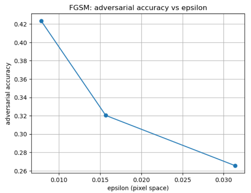
# plot
plt.figure()
plt.plot([r["eps_pixel"] for r in results], [r["adv_acc"] for r in results], marker='o')
plt.xlabel("epsilon (pixel space)")
plt.ylabel("adversarial accuracy")
plt.title("FGSM: adversarial accuracy vs epsilon")
plt.grid(True)
plt.show()
The results are shown below:
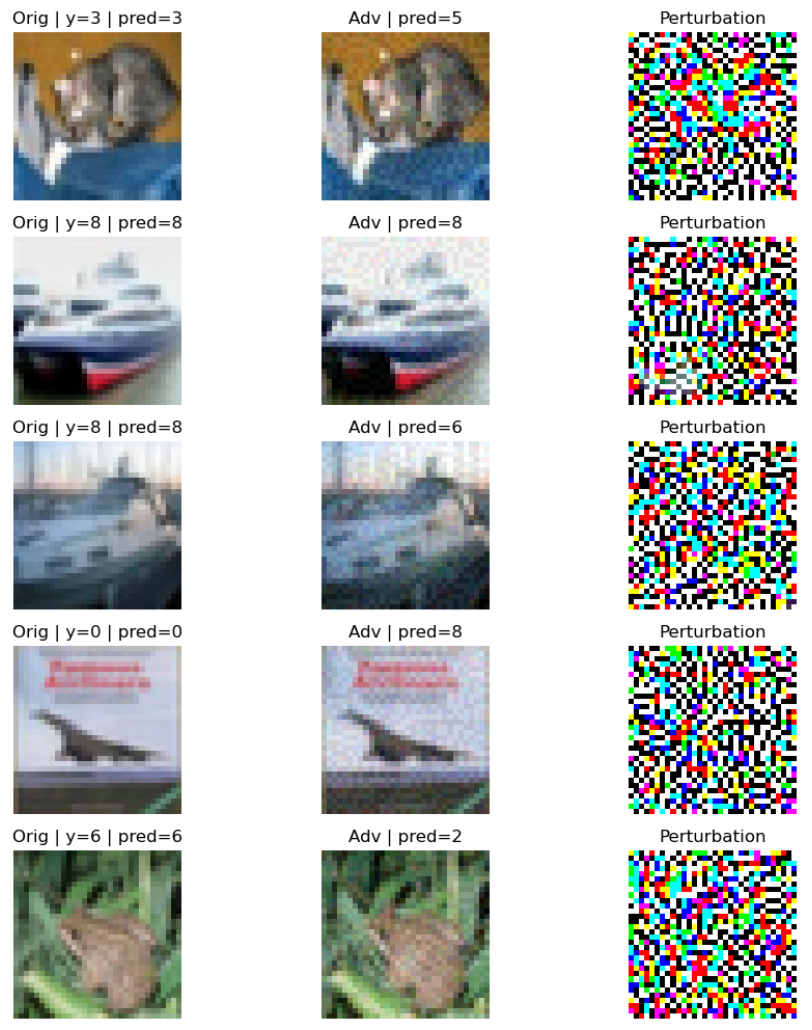
FGSM Visualization:
# === FGSM visualization (provided) ===
import numpy as np
import matplotlib.pyplot as plt

def imshow(img):
    # undo normalization (assumes Normalize(0.5,0.5,0.5))
    img = img.detach().cpu().numpy()
    img = (img * 0.5) + 0.5
    npimg = np.transpose(img, (1, 2, 0))
    return np.clip(npimg, 0, 1)

# pick a batch
dataiter = iter(testloader)
images, labels = next(dataiter)
images, labels = images.to(device), labels.to(device)

# choose epsilon (pixel space) and convert if normalized
eps_pixel = 8/255
eps = eps_pixel / 0.5

# generate adversarial examples
adv_images, perturbation = fgsm_attack(model, images, labels, eps, device)

# predictions
with torch.no_grad():
    pred_clean = model(images).argmax(dim=1)
    pred_adv = model(adv_images).argmax(dim=1)

# show first 5
k = 5
plt.figure(figsize=(10, 2*k))
for i in range(k):
    orig = imshow(images[i])
    adv  = imshow(adv_images[i])

    pert = (adv_images[i] - images[i]).detach().cpu().numpy()
    pert = (pert - pert.min()) / (pert.max() - pert.min() + 1e-8)
    pert = np.transpose(pert, (1, 2, 0))

    plt.subplot(k, 3, 3*i+1)
    plt.imshow(orig); plt.axis('off')
    plt.title(f"Orig | y={labels[i].item()} | pred={pred_clean[i].item()}")

    plt.subplot(k, 3, 3*i+2)
    plt.imshow(adv); plt.axis('off')
    plt.title(f"Adv | pred={pred_adv[i].item()}")

    plt.subplot(k, 3, 3*i+3)
    plt.imshow(pert); plt.axis('off')
    plt.title("Perturbation")

plt.tight_layout()
plt.show()
The results are shown below:
PGD Attack Example
Review of Principles
Untargeted PGD:
Targeted PGD:
.
Pseudocode
Let us look at how to carry out a complete PGD attack in practice:
[INPUT]
Model (parameters fixed, not updated)
Original image x, pixel range assumed to be -1 to 1
Maximum perturbation epsilon, L_inf constraint
Step size alpha
Number of iterations T
Attack target: y or y_t

Optional: random initialization
Optional: PNG/uint8 quantization: QAA/STE, etc.

[INITIALIZATION]
Copy the original image as x0, ensuring it does not participate in gradient updates (treated as a constant)
Initialize perturbation delta: if using random initialization, sample delta uniformly from [-epsilon, +epsilon]; otherwise delta = 0
Set adversarial example x_adv = clamp(x_0 + delta, 0, 1) to ensure valid pixel values
If quantization-aware mode is enabled, quantize x_adv to the k/255 grid, then back-compute delta = x_adv - x_0 to start on the PNG grid
Prepare to track the best result: best_loss = float('inf'), best_delta = float('inf')

[ITERATIVE OPTIMIZATION]
Repeat T times:
    Generate current adversarial example x_adv = clamp(x_0 + delta, 0, 1)
    (If using QAA/STE, use the quantized image in the forward pass but let gradients flow as if no quantization occurred in the backward pass)
    Forward pass to compute loss
        For classification tasks: loss = CrossEntropy(model(x_for_loss), y or y_t)
        For multimodal tasks: loss = AttackLoss(model, x_for_loss, target_text)
    Record current best loss
    Backward pass to obtain gradients
        First clear old gradients
        loss.backward() to get g = dL/d_delta
    FGSM-style perturbation update
        If targeted: delta = delta - alpha * sign(g)
        If untargeted: delta = delta + alpha * sign(g)
    Projection / Clipping
        First ensure perturbation magnitude does not exceed epsilon: delta = clamp(delta, -epsilon, +epsilon)
        Then ensure pixels remain in [0, 1]: delta = clamp(x0 + delta, 0, 1) - x0
    (If using quantization-aware mode, snap to uint8 grid at each step to improve PNG robustness)
        x_snap = round(clamp(x0 + delta, 0, 1) * 255) / 255
        delta = x_snap - x0

[OUTPUT]
Generate the final adversarial example using the best perturbation: x_adv_final = clamp(x0 + best_delta, 0, 1)
If quantization-aware mode is enabled, apply a final quantization: x_adv_final = round(x_adv_final * 255) / 255
RETURN: x_adv_final, best_delta (and optionally the loss curve)
.
ViT Injection Attack Example
We use Qwen2.5-VL-3B-Instruct as an example to perform a text injection attack. A simplified view of the Qwen2.5-VL-3B-Instruct (hereafter Qwen2.5VL) architecture:
Input Image (H×W×C)
  ↓
Split into patches (P×P) → N patches
  ↓
Linear projection to D-dim tokens  (N×D)
  ↓
Add positional embedding (+ optional [CLS])
  ↓
Transformer Encoder × L
  - (Window) Multi-head self-attention
  - MLP (SwiGLU/GELU)
  - Norm + residual
  ↓
Output visual token sequence (N×D) / or CLS for classification
The input image is split into patches of size P, each patch is encoded as an embedding of length D, and these are then fed into the transformer as a sequence.
To make the output text contain or match a target_text, there are two mainstream injection approaches:
- Traditional PGD perturbation — iteratively perturbing image pixels so that the model's generation probability distribution shifts toward the target text.
- Visual prompt injection — embedding instructions as part of the input content (readable text in the image, metadata, etc.) to exploit the model's instruction-following mechanism and alter its behavior (no gradient required).
The first approach works by optimizing a target text loss:
Targeted PGD:
Or in iterative update form:
Visual/multimodal prompt injection, on the other hand, uses "instructions" as contextual content to mislead the model. This approach typically does not involve differentiable optimization of pixels. Instead, it is more about selecting an injection string \(s\) (such as readable text in the image or instructions the model will extract) that makes the model more likely to produce the attacker's desired output \(y^*\).
After context injection, the attacker aims to maximize the probability of the target output:
If we want to emphasize that "the model first extracts text/content from the image before reasoning," we can write:
Here \(E(\cdot)\) represents "the representation the model derives from the image / the text extracted / the visual semantics" (not necessarily explicit OCR, but conceptually the image information entering the context/conditioning).
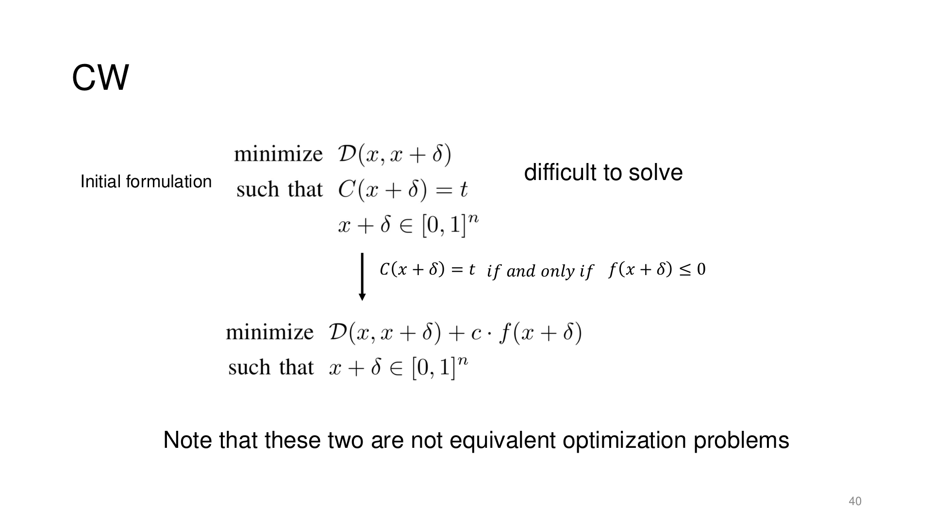
Source: Tufts EE141 Trusted AI, Lecture 3, Slide 40. Image note: the slide shows how the C&W attack relaxes a hard-constraint classification problem into a differentiable optimization. Why it matters: C&W is stronger than FGSM/PGD because it directly optimizes classification confidence rather than loss — this constraint-relaxation technique is key to understanding modern optimization-based attacks.
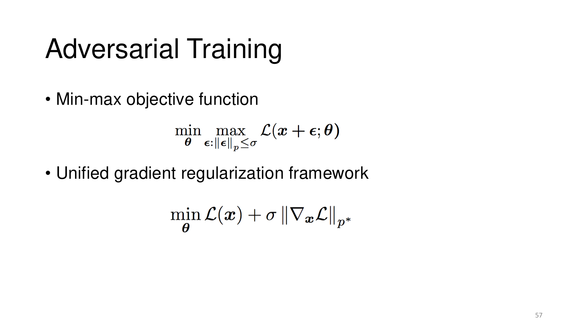
Source: Tufts EE141 Trusted AI, Lecture 3, Slide 57. Image note: the slide casts adversarial training as a min-max objective and shows its equivalent gradient-regularization form. Why it matters: adversarial training is not an ad-hoc trick but a rigorous robust-optimization problem.