Graph Theory

Graph theory problems pervade all of computer science, and graph algorithms are of critical importance.

Images are sourced from the internet and not all sources could be attributed. They are not used for any commercial purpose.

Common algorithm quick reference:

Name	App	DS	Time	Space
BFS	UnWtd	Queue	\(O(V+E)\)	\(O(V)\)
DFS	Connectivity	Stack / Recursion	\(O(V+E)\)	\(O(V)\)
Dijkstra	SSSP	Binary Heap	\(O((V+E) \log V)\)	\(O(V+E)\)
	Non-neg	Fibonacci Heap	\(O(E + V \log V)\)	\(O(V+E)\)
Bm-Fd	SSSP Neg√	E-1 loops for longest possible	\(O(V \cdot E)\)	\(O(V)\)
Flyd-W	APSP	DynamicPrg	\(O(V^3)\)	\(O(V^2)\)
Kruskal	MST	DSU+ Sorting	\(ElogE+E \alpha (V)\)	\(O(V+E)\)
Prim	MST	Binary Heap	\(O((V+E) \log V)\)	\(O(V+E)\)
		Fibonacci Heap	\(O(E + V \log V)\)	\(O(V+E)\)
TopoSt	DAGs	Stack (DFS)	\(O(V+E)\)	\(O(V+E)\)

.

Graph Representation

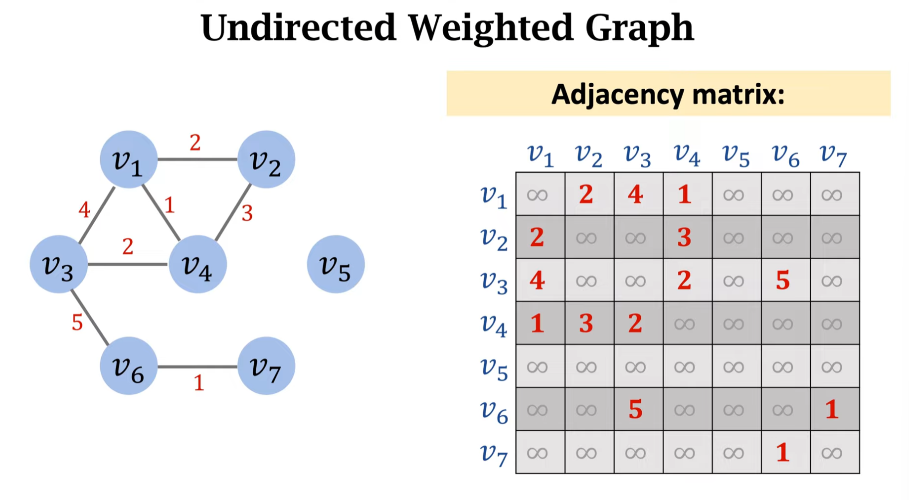
For a graph \(G=(V, E)\), we use G.V to denote the vertex set and G.E to denote the edge set.

There are several common ways to represent a graph:

• Drawing the graph directly
• Adjacency List
• Adjacency Matrix

In most cases, we use an adjacency list to represent a graph, because most graphs are sparse (\(E\) is much smaller than \(V^2\)). Only for dense graphs (\(E\) is close to \(V^2\)) is an adjacency matrix more appropriate.

Note that in practice, adjacency lists have two main representations:

• In Python, use a dict to represent the adjacency list
• In Python, use List[List[]] to represent the adjacency list

For example, for a directed graph:

{
  "a": ["c", "d"],
  "b": ["a", "c"],
  "c": ["d"],
  "d": ["e"],
  "e": ["a"]
}

In this graph, a points to c and d, and the rest follow the same pattern. We can summarize the following information:

• \(V\) (Vertex Set): $$ V = {a, b, c, d, e} $$
• \(E\) (Edge Set): (note the direction of the arrows) $$ E = {(b, a), (b, c), (a, c), (a, d), (c, d), (d, e), (e, a)} $$
• Statistics: \(|V| = n = 5\) (number of vertices), \(|E| = m = 7\) (number of edges)

For an undirected graph:

{
  "a": ["b", "c", "d", "e"],
  "b": ["a", "c"],
  "c": ["a", "b", "d"],
  "d": ["a", "c", "e"],
  "e": ["a", "d"]
}

From the above, we can see that a's neighbors include e, and e's neighbors include a, meaning a and e point to each other. We can extract the following information:

• \(V\) (Vertex Set): $$ V = {a, b, c, d, e} $$
• \(E\) (Edge Set): $$ E = {(a, b), (a, c), (a, d), (a, e), (b, c), (c, d), (d, e)} $$

Related graph terminology includes:

Term	Definition
Vertices
Edges
Adjacent	Two vertices are adjacent if they are connected by an edge.
Neighbor	All vertices adjacent to a given vertex are called its neighbors.
Directed	Whether one vertex points to another.
Weighted
Incident	An edge is incident to a vertex if it connects to that vertex.
Degree	The number of edges connected to a vertex.
Path	A sequence of edges and vertices from one vertex to another.
Simple Path	A path in which no vertex is repeated.
Distance / Length	The number of edges in the shortest path from one vertex to another.
Cycle	A path whose start and end vertices are the same, containing at least three vertices.
Acyclic
Simple Cycle	A cycle that does not repeat any vertex except the start.
Connected	A graph is connected if there exists a path between any two vertices.
Component	A maximal connected subgraph.

Based on the definition and properties of graphs, we can observe:

• A tree is a special graph (acyclic with n-1 edges, or acyclic and connected).
• In an undirected graph, each edge contributes 1 to the degree of each of its two endpoints, so the sum of all vertex degrees equals twice the number of edges.
• A graph with n vertices has a minimum of 0 edges; such a graph is called a totally disconnected graph.
• The minimal connected acyclic graph is a tree.
• The maximum number of edges occurs in a complete graph, where every pair of distinct vertices is connected by an edge, giving n*(n-1)/2 edges.

---

A tree is essentially a connected, acyclic, undirected graph.

For an undirected graph \(T\) with \(n\) vertices, it is defined as a tree if it satisfies any one of the following conditions. These four properties are mathematically equivalent (each is a necessary and sufficient condition for the others).

1. Edge count property: \(T\) is connected and has exactly \(n - 1\) edges.
   • Explanation: If you have 5 vertices, connecting them without forming a cycle requires exactly 4 edges.
2. Minimal connectivity: \(T\) is connected, but removing any single edge \(e\) from \(T\) disconnects the graph.
   • Explanation: This means the tree has no redundant edges (i.e., no cycles). Every edge is a necessary "bridge" for maintaining connectivity.
3. Acyclicity property: \(T\) is a connected graph with no cycles.
   • Explanation: This is the most intuitive definition of a tree: connected and loop-free.
4. Unique path: Between any pair of vertices in \(T\), there exists exactly one simple path.
   • Explanation: If there were two paths, a cycle would form; if there were no path, the graph would be disconnected.

Directed and Undirected Graphs

For any graph, we should quickly identify:

• Whether it is directed: directed graph / undirected graph
• Whether it is weighted: weighted graph / unweighted graph

For a directed graph, two important concepts are:

• Strongly Connected Components (SCC)
• Directed Acyclic Graph (DAG)

For an undirected graph, several important concepts are:

• Connected Components
• Cut Vertices (Articulation Points)
• Bridges (Cut Edges)

It is essential to distinguish between these concepts for directed and undirected graphs.

---

Strongly Connected Components (SCC) apply only to directed graphs:

In a directed graph, if u can reach v and v can also reach u (mutually reachable), then u and v belong to the same strongly connected component.

In other words, they must be mutually reachable:

• There exists a directed path from u to v
• There exists a directed path from v to u

For details on finding SCCs, see the dedicated SCC section.

---

Directed Acyclic Graphs (DAGs) are a frequently discussed type of graph. For example, an AOV network (Activity On Vertex Network) is a DAG.

Topological sorting can be performed on a DAG:

Topological sorting is a linear ordering of the vertices of a directed graph such that for every directed edge \((u, v)\), vertex \(u\) appears before vertex \(v\) in the ordering.

Only DAGs can be topologically sorted. If a directed graph contains a cycle, then no linear ordering of the vertices on that cycle can satisfy the topological sort requirement. For example, in the cycle \(A \to B \to C \to A\), if \(A\) comes before \(B\), then \(B\) must come before \(C\), and \(C\) must come before \(A\), which is a contradiction. Therefore, being a DAG is a necessary and sufficient condition for topological sorting.

Both BFS and DFS can be used to implement topological sorting.

For details on DAGs, see the BFS Topological Sort or DFS Topological Sort sections.

For graphs with cycles, by finding SCCs and compressing each SCC into a single vertex, a cyclic directed graph can be converted into a DAG. See the appendix for related exercises.

---

Connected Components are maximal connected subgraphs of an undirected graph:

In an undirected graph, if there exists a path between two nodes (regardless of the route), they belong to the same connected component.

For example:

A -- B -- C      D -- E

In the graph above, there are two connected components: A-B-C and D-E. Note that although A-B within A-B-C is also connected, it is not a complete connected component, because a connected component is the largest set of mutually reachable nodes in an undirected graph.

---

Cut Vertices & Bridges

A cut vertex (articulation point) applies only to undirected graphs. Its simple definition is: removing that vertex increases the number of connected components. Equivalently: in a connected graph, if removing a vertex makes the graph disconnected, that vertex is a cut vertex.

A bridge (cut edge) is an edge whose removal disconnects the undirected graph.

For details, see Tarjan's Algorithm for Cut Vertices/Bridges.

Weighted and Unweighted Graphs

A graph without edge weights is called an unweighted graph; a graph with edge weights is called a weighted graph.

For undirected weighted graphs, the weight of non-existent edges is typically treated as 0 or infinity. If we think of each vertex as a node in a network:

• If edges represent bandwidth, edge = 0 means not connected
• If edges represent network latency, edge = infinity means unreachable or servers are not connected

The same principle applies to directed weighted graphs.

An unweighted graph can be viewed as a special weighted graph where all weights are 1 or uniform.

Dense and Sparse Graphs

A dense graph is one whose edge count (\(E\)) approaches the maximum possible number of edges; conversely, a graph with very few edges is called a sparse graph.

The graph density \(D\) is the ratio of the actual number of edges to the maximum possible number of edges, with a range of \(0 \le D \le 1\). Specifically:

• \(D = 1\): Complete graph, the densest possible graph.
• \(D = 0\): A graph with no edges.

Let \(|E|\) denote the number of edges and \(|V|\) denote the number of vertices. Then:

For undirected simple graphs, the maximum number of edges is \(\binom{|V|}{2} = \frac{|V|(|V|-1)}{2}\), and the density formula is:

\[ D = \frac{2|E|}{|V|(|V|-1)} \]

For directed simple graphs, the maximum number of edges is twice that of undirected graphs (because each edge has two possible directions). The density formula is:

\[ D = \frac{|E|}{|V|(|V|-1)} \]

In computer science, determining whether a graph is dense or sparse does not always rely on a precise "density threshold" (e.g., density > 0.5 means dense). Instead, it is primarily based on the order-of-magnitude relationship between edge count \(|E|\) and vertex count \(|V|\), as well as which data structure or algorithm is more efficient for the given scenario:

• Asymptotic complexity: Judge based on the graph's growth scale and edge growth trends.
• Space efficiency: When \(|E| \ll |V|^2\), an adjacency list is usually more efficient, and the graph is considered sparse.
• Time complexity: If an \(O(|V|^2)\) algorithm runs faster than an \(O(|E| \log |V|)\) algorithm, the graph is dense.
• Rule of thumb: Generally, when D < 10%, an adjacency list is the default; when D > 30%, an adjacency matrix is preferred.

Breadth-First Search (BFS)

Breadth-First Search (BFS) is the simplest graph search algorithm and serves as the prototype for many important graph algorithms (such as Prim's MST and Dijkstra's shortest path, discussed later). It is called BFS because the algorithm must discover all nodes at distance k from the source before discovering any node at distance k+1.

To track progress, BFS typically marks nodes that have been visited. Conceptually, this is often represented by coloring nodes; in practice, a visited set is used for bookkeeping.

During BFS execution, a BFS tree is constructed. Initially, the BFS tree contains only the root, which is the source node s. When scanning the neighbors of a discovered node u, whenever a new unvisited node v is found, the edge (u, v) is added to the BFS tree. In the BFS tree, u is the predecessor (or parent node) of v. Since each node is discovered at most once, each node has at most one parent.

In CLRS, colors are used to distinguish node states:

• White: unvisited node
• Gray: visited node whose neighbors have not all been examined
• Black: visited node whose neighbors have all been discovered

The pseudocode is as follows:

BFS(G, s)
1  for each vertex u ∈ G.V - {s}
2      u.color = WHITE
3      u.d = ∞
4      u.π = NIL    | Set to NIL because all parent nodes are initially undiscovered
5  s.color = GRAY
6  s.d = 0
7  s.π = NIL
8  Q = ∅
9  ENQUEUE(Q, s)
10 while Q ≠ ∅
11     u = DEQUEUE(Q)
12     for each v ∈ G.Adj[u]
13         if v.color == WHITE
14             v.color = GRAY
15             v.d = u.d + 1
16             v.π = u
17             ENQUEUE(Q, v)
18     u.color = BLACK

In practice, a single visited set suffices to track all visited nodes. The Python implementation is as follows:

from collections import deque

def BFS(graph, start):
    queue = deque([start]) # 使用 deque 作为队列，性能 O(1)

    # 如果不需要存储距离，则直接用一个set visited记录已经访问过的点就可以了
    distances = {start: 0}

    parents = {start: None} # 记录路径 (前驱节点)

    # 主循环
    while queue:
        current = queue.popleft()  # 取出队首 (相当于 DEQUEUE)

        # 遍历邻居
        for neighbor in graph[current]:
            if neighbor not in distances:
                distances[neighbor] = distances[current] + 1
                parents[neighbor] = current
                queue.append(neighbor) # 加入队尾 (相当于 ENQUEUE)

    return distances, parents

# =================测试=================
# 同样的图结构
G = {
    'r': ['s', 'v'], 's': ['r', 'w'], 't': ['w', 'x', 'u'],
    'u': ['t', 'x', 'y'], 'v': ['r'], 'w': ['s', 't', 'x'],
    'x': ['w', 't', 'u', 'y'], 'y': ['x', 'u']
}

dists, paths = BFS(G, 's')

print("节点 | 最短距离 | 父节点")
for node in G:
    # 使用 .get() 防止图中有些点可能从起点无法到达（属于非连通图）
    d = dists.get(node, '不可达')
    p = paths.get(node, '无')
    print(f" {node}   |    {d}     |   {p}")

As you can see, the Python code is even more concise than the pseudocode. For subsequent sections, we will use Python directly for code examples.

The time complexity of BFS is \(O(V+E)\).

---

BFS Tree

If we record the parent of each node during BFS, we obtain the BFS tree. This tree is very useful for:

• Finding shortest paths: In an unweighted graph, the path from the root to any node in the BFS tree is the shortest path.
• Determining hierarchical relationships: In applications like six degrees of separation and LinkedIn social networks, the BFS tree quickly reveals how many people separate A from B (i.e., computing the Kevin Bacon Number).

However, if we build a BFS tree rooted at A and then want to know the distance from C to D, we must rebuild a new BFS tree rooted at C. Therefore, BFS is a single-source shortest path algorithm. If we want to know all-pairs shortest paths (i.e., the distance between every pair of vertices), we need to run BFS from every vertex (assuming an unweighted graph). More on single-source and all-pairs shortest paths will be discussed later.

Topological Sort (Kahn's Algorithm)

Kahn's Algorithm is a very popular and intuitive method for implementing topological sorting, based on the idea of breadth-first search (BFS) and using vertex in-degrees.

A point that is easily overlooked about DAGs:

A DAG can contain isolated vertices.

The core principle of topological sorting is:

For every directed edge \(u \to v\) in the graph, vertex \(u\) must appear before vertex \(v\) in the ordering.

Let us consider an isolated vertex D:

• D has no incoming edges (in-degree = 0): This means it depends on no other node in the graph. Therefore, it does not need to wait for any node to be sorted before it can be placed.
• D has no outgoing edges (out-degree = 0): This means it constrains no other node in the graph. No node is required to appear after D.

Since D has no dependencies and is not depended upon, its position in the topological sort is free and will not violate any constraints.

The reason we specifically mention DAGs and isolated vertices is that in Kahn's algorithm, isolated nodes must be (or rather, will naturally be) considered, but they require no special handling. In practice, we typically build the graph first, updating in-degree values along the way. When enqueuing, we must check the in-degree of all vertices in the graph.

---

The logic of Kahn's algorithm is very intuitive: in a DAG, any task (vertex) with no prerequisites (i.e., in-degree 0) can be executed first. Therefore, Kahn's algorithm continuously finds vertices with in-degree 0, removes them from the graph (i.e., removes them from the processing queue and decrements their neighbors' in-degrees), until all vertices have been processed.

In other words, our goal is topological sorting, so we first identify the "root-level" vertices -- those with no predecessors. Each time we find such a vertex, its neighbors' in-degrees decrease by one, because the found vertex is already placed in the result list and no longer needs to be considered as a predecessor.

Here is the algorithm outline:

Kahn's Algorithm

# Compute in-degree for all vertices
Traverse all edges (u, v) in G, counting how many edges point to v

# Initialize queue
Create a queue Q
Traverse all vertices, enqueuing all vertices with in-degree 0

# BFS loop
While queue Q is not empty:
    Dequeue: Remove a vertex u from Q, add it to the topological sort result list
    Traverse all neighbors v of u:
        Decrement v's in-degree by 1
        If v's in-degree drops to 0, all of v's prerequisites are satisfied; enqueue v

# Check for cycles
If the result list contains as many vertices as the total vertex count V, the graph is a DAG
Otherwise (fewer vertices than V), the graph contains a cycle

The time complexity of Kahn's algorithm is O(V+E), since it computes the in-degree of each vertex once and visits each edge once to perform the in-degree decrement.

As we can see, Kahn's algorithm not only provides convenient and fast sorting but can also be used to detect cycles.

During graph DFS, we similarly use three colors to represent three states:

• White (WHITE): unvisited
• Gray (GRAY): on the recursion stack (currently being visited)
• Black (BLACK): finished processing

When first exploring edge \((u, v)\), we can determine the edge type based on \(v\)'s color:

Color of v	Edge Type
White	Tree Edge
Gray	Back Edge
Black	Check timestamps to determine: Forward Edge or Cross Edge

Tree edges, back edges, forward edges, and cross edges:

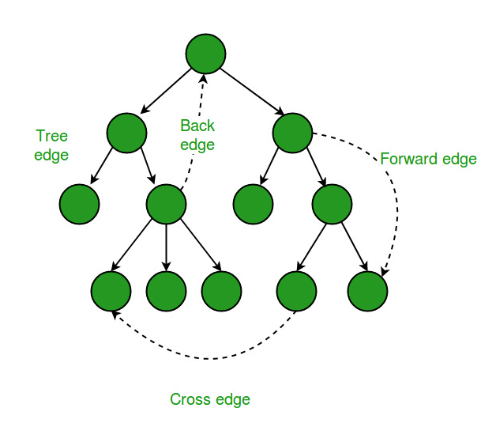
In undirected graphs, only tree edges and back edges occur.

Depth-First Search (DFS)

DFS Tree

Depth-first search (DFS) is extremely important in graph theory and gives rise to numerous techniques and algorithms. When DFS starts from a source vertex \(u\) and recursively descends into other nodes, forming branches, the tree produced during this process is called a DFS tree. When the graph is disconnected, multiple DFS trees are formed, creating a DFS forest. During DFS, the moment a node transitions from unvisited to visited is called discovering that node.

During DFS, each node \(v\) records the node from which it was discovered; this parent node is called its predecessor (or parent). Since each node's predecessor is determined the first time DFS visits it, each node has at most one predecessor. The predecessor relationships in DFS define the edges of the DFS tree. All nodes' predecessor pointers form a predecessor subgraph.

During DFS, each node records two timestamps:

• Discovery time: d[v] -- the time when a node is first discovered
• Finish time: f[v] -- the time when all of a node's neighbors have been fully processed

Note that if a node has no neighbors after being discovered, its finish time still increments by one, as shown below:

Clearly, for every node \(u\):

\[ u.d < u.f \]

.

---

Let us illustrate with an example. Consider the following directed graph:

       A → B → C
       |   |   |
       v   v   v
       D → E → F

The adjacency list for this graph is:

Adj[A] = [B, D]
Adj[B] = [C, E]
Adj[C] = [F]
Adj[D] = [E]
Adj[E] = [F]
Adj[F] = [ ]

Performing DFS starting from A:

• First visit A
• Then visit B (from A)
• Then visit C (from B)
• Then visit F (from C); F has no neighbors, F finishes
• Return to C; F is done, no unvisited neighbors remain, C finishes
• Return to B; visit the next unvisited neighbor E
• E's only neighbor is F, which has already been visited, so E finishes
• Return to B; all neighbors are done, B finishes
• Return to A; visit A's second neighbor D
• D finishes
• A finishes

Adding timestamps, we get the following table:

Node	d[v]	f[v]
A	1	12
B	2	9
C	3	6
F	4	5
E	7	8
D	10	11

We also obtain the predecessor table:

Node	parent
A	NIL
B	A
C	B
F	C
E	B
D	A

Connecting the parent pointers gives us the predecessor subgraph (DFS tree):

        A
       / \
      B   D
     / \
    C   E
    |
    F

.

---

Finally, let us look at the DFS pseudocode and implementation:

def DFS(G):
    """
    G: 邻接表形式的图，例如：
        G = {
            'A': ['B', 'D'],
            'B': ['C', 'E'],
            ...
        }
    返回:
        color  : 颜色(white/gray/black)
        d      : 发现时间
        f      : 完成时间
        parent : 前驱指针(构成 DFS 树/森林)
    """
    color  = {}
    d      = {}
    f      = {}
    parent = {}

    # 初始化
    for u in G:
        color[u]  = 'white'
        parent[u] = None

    time = 0  # 全局时间戳

    def dfs_visit(u):
        nonlocal time
        time += 1
        d[u] = time          # 发现时间
        color[u] = 'gray'    # 变灰色（正在处理）

        for v in G[u]:
            if color[v] == 'white':
                parent[v] = u
                dfs_visit(v)

        color[u] = 'black'   # 处理完成
        time += 1
        f[u] = time          # 完成时间

    # 可能是非连通图，因此要遍历所有结点，得到 DFS 森林
    for u in G:
        if color[u] == 'white':
            dfs_visit(u)

    return color, d, f, parent

# 使用示例
G = {
    'A': ['B', 'D'],
    'B': ['C', 'E'],
    'C': ['F'],
    'D': ['E'],
    'E': ['F'],
    'F': []
}

color, d, f, parent = dfs(G)

.

Euler Tour

The Euler Tour can be understood as an enhanced version of timestamps.

In the timestamp approach, we record each node's discovery and finish times, making it easy to determine whether one node is an ancestor of another. Specifically, if \(v\) is in \(u\)'s DFS subtree, then:

\[ d[u] < d[v] < f[v] < f[u] \]

The above is equivalent to saying: \(u\) is an ancestor of \(v\). This property arises from the nesting nature of timestamp intervals:

• An interval opens when a node is first visited
• The interval closes when backtracking leaves that node
• All nodes in the subtree must have their intervals opened and closed within the parent's interval
• If \(v\) is a descendant of \(u\), DFS must visit \(v\) while processing \(u\)
• If \(v\) is visited during the recursive processing of \(u\), then \(u\) must be an ancestor of \(v\)

If we record the visit order during DFS, including revisits, we obtain the Euler tour.

---

For example, consider the following directed graph:

1: [2, 3]
2: [4, 5]
3: [5]
4: [2, 6]
5: [4]
6: [3]

Starting from vertex 1, we construct the DFS tree and record timestamps:

Node u	d[u]	f[u]
1	1	12
2	2	11
4	3	10
6	4	9
3	5	8
5	6	7

From the timestamps, we can easily determine the DFS tree structure:

1
└── 2
    └── 4
        └── 6
            └── 3
                └── 5

Now we can extract many key insights. For example, in the DFS tree, node 4's timestamp interval is nested within node 1's interval, so 1 is an ancestor of 4.

Furthermore, in a directed graph DFS, if an edge \(u \to v\) is encountered where \(v\) has already been visited and \(v\) is still on the current DFS recursion stack (i.e., colored gray), then this edge is a back edge. We can use timestamps to identify back edges directly. For instance, when DFS reaches node 4 via nodes 1 and 2, node 4's neighbor list contains 2, and we are currently within 2's recursion, so \(4 \to 2\) is a back edge.

We can use timestamps to check: in a directed graph, for a directed edge \(a \to b\), if:

\[ d[b] < d[a] < f[a] < f[b] \]

then \(a \to b\) is a back edge. This is because:

• b is an ancestor of a
• a points to b

Therefore, the edge from a to b is a back edge, and the directed graph contains a cycle.

---

During the DFS above, we record every visited node, including revisits, forming the Euler tour:

[1, 2, 4, 6, 3, 5, 5, 3, 6, 4, 2, 1]

Using the Euler tour, we can easily find the Lowest Common Ancestor (LCA) of two nodes. For the Euler tour above, if we want to find the LCA of 5 and 6:

Index:   1  2  3  4  5  6  7  8  9  10 11 12
Euler = [1, 2, 4, 6, 3, 5, 5, 3, 6, 4, 2, 1]

There are 12 elements. We can see:

• The first occurrence of 5 is at index 6, i.e., first[5] = 6
• The first occurrence of 6 is at index 4, i.e., first[6] = 4

We take the interval of the Euler tour:

• Euler[4..6] = [6, 3, 5]

We also need to consider depth. Writing out the depths:

Euler:  1  2  4  6  3  5  5  3  6  4  2  1
Depth: [0, 1, 2, 3, 4, 5, 5, 4, 3, 2, 1, 0]
Index:   1  2  3  4  5  6  7  8  9 10 11 12

Within the interval [4, 6], the nodes and depths are:

index	node	depth
4	6	3
5	3	4
6	5	5

The node with the minimum depth is 6, so 6 is the LCA.

This gives us a general solution for the LCA problem:

LCA(u, v) = the node with the minimum depth in the Euler tour between first[u] and first[v].

Parenthesis Theorem

The Parenthesis Theorem is the theoretical foundation for many graph algorithms, primarily used to analyze DFS timestamps, ancestor relationships, and edge types.

In any DFS of a directed or undirected graph, for any two nodes u and v, exactly one of the following three cases holds:

1. The two intervals are completely disjoint, i.e., \([d[u], f[u]]\) and \([d[v], f[v]]\) do not overlap at all
2. \(u\)'s interval completely contains \(v\)'s interval
3. \(v\)'s interval completely contains \(u\)'s interval

From this theorem, the following important corollaries can be derived:

• When \(u\)'s interval completely contains \(v\)'s interval, \(u\) is an ancestor of \(v\)
• If \(u\) is an ancestor of \(v\), then DFS must visit \(v\) during \(u\)'s recursive processing

We can also derive the White-Path Theorem:

If \(u\) is an ancestor of \(v\), then there exists a path from \(u\) to \(v\) consisting entirely of white (unvisited) nodes.

These theorems are applied in the following concepts:

• Determining ancestor/descendant relationships in DFS trees
• Detecting cycles in directed graphs (i.e., identifying back edges)
• Proving the correctness of topological sorting
• Strongly connected components
• Finding bridges and articulation points

Topological Sort (DFS Version)

Although BFS-based topological sort is more commonly used, for a graph that is confirmed to be a DAG, the DFS approach is actually quite straightforward:

1. Pick any vertex (e.g., in lexicographic order) as the starting point for DFS
2. During DFS, a node can only be pushed to the result after all its neighbors have been pushed
3. Reverse the result to obtain the topological sort

The DFS topological sort process is also used when computing SCCs; see the SCC section on Kosaraju's Algorithm.

For a graph confirmed to be a DAG, the DFS algorithm is very simple:

DFS Topological Sort for a confirmed DAG

result = []
visited = set()

def DFS(vertex):
    Traverse vertex's neighbors:
        If neighbor not in visited:
            DFS(neighbor)
    result.append(vertex)

REVERSE result

However, in real-world problems, we often cannot be sure whether a graph has cycles, so merely tracking whether a node has been visited is insufficient.

During graph DFS, we typically use three colors for three states:

• White (WHITE): unvisited
• Gray (GRAY): on the recursion stack (currently being visited)
• Black (BLACK): finished processing

Alternatively, if colors are hard to remember, states can be used:

• Unvisited: visited = "unvisited"
• Visiting: visited = "visiting"
• Visited: visited = "visited"

Clearly, while performing DFS on a vertex:

• If we encounter a neighbor in the "visiting" state, the graph is not a DAG and topological sorting is impossible

Here is the complete DFS algorithm:

DFS Topological Sort

Initialize graph
Set up three states: unvisited, visiting, visited
Set all vertices to unvisited

DFS(vertex):
    Set vertex state to visiting
    Traverse vertex's neighbors:
        If a neighbor is visiting:
            Cycle detected; topological sort is meaningless; handle as desired
            Typically I set a CYCLE=True flag here
        If a neighbor is unvisited:
            DFS(neighbor)
    Set vertex state to visited
    Add vertex to result

Visit all vertices:
    If vertex state is unvisited:
        DFS(vertex)
    If CYCLE==True:
        Terminate early; result is invalid

REVERSE result to get the topological sort

The time complexity of DFS-based topological sorting is \(O(V+E)\).

Tarjan's Algorithm for Cut Vertices/Bridges

Tarjan is an expert in graph theory who proposed three famous algorithms built upon DFS:

• Tarjan's SCC Algorithm (for strongly connected components)
• Tarjan's algorithm for articulation points (for cut vertices)
• Tarjan's algorithm for bridges

As a side note, the Fibonacci heap is also one of Tarjan's contributions.

This section focuses on using Tarjan's algorithm to find cut vertices and bridges. For SCCs, see the SCC section.

In my notes, the two Tarjan algorithms for undirected graphs are referred to as "Tarjan Cut" (a name I coined to distinguish them from Tarjan SCC). Tarjan Cut is for undirected graphs.

The two core elements of Tarjan's algorithm are:

• DFS
• Lowlink value

Let us first look at the DFS part, which is easier to understand:

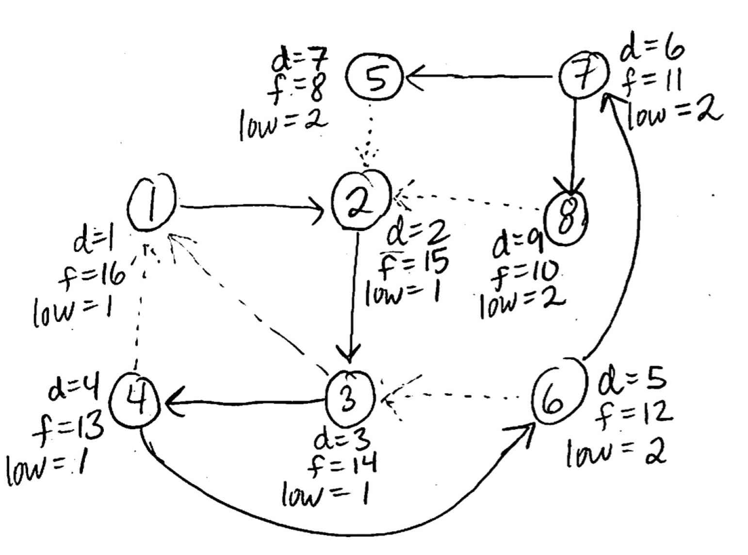
We perform a DFS on the undirected graph. Starting from some vertex, each time we visit a new vertex, we assign it a timestamp representing its discovery time. Note that we only record the first visit time, not the leaving time. We use a global counter time, incrementing it each time a new vertex is visited: dfn[u] = ++time. Each vertex's first discovery time is called its Depth-First Number, commonly abbreviated as dfn.

---

Next, let us examine the lowlink value. The low-link value (commonly abbreviated as low) is the core of Tarjan's algorithm -- its very soul.

In simple terms, low[u] represents the earliest ancestor reachable from u's subtree. Let us first understand what "jumping up" means. Normally in DFS, we always descend from parent to child:

Parent
 ↓
Child
 ↓
Grandchild

To return to a higher node (closer to the root), we normally need to backtrack. However, since the tree structure here is not derived from an inherent tree but rather is a DFS tree generated from a graph structure, at any depth we might suddenly jump back to a shallower position. This is "jumping up" -- essentially what we earlier called a back edge.

With an understanding of jumping up, let us look at the lowlink value. In brief, the low value tells us during DFS tree backtracking whether a node can reach back to an ancestor through its subtree. If it can, there exists a back edge that forms a cycle or strongly connected structure involving the node, its subtree, and its ancestor.

This may sound convoluted, so let us look at a specific example:

1
|
2 <- 5
|
3
|
4
|
5 -> 2

In the above, vertex 5 has a back edge directly to vertex 2. Clearly, during DFS we visit vertices 1 through 5 in order, so the dfn values are straightforward:

dfn[1] = 1
dfn[2] = 2
dfn[3] = 3
dfn[4] = 4
dfn[5] = 5

During DFS, whenever a new node is visited, at that moment the node itself is the earliest ancestor it can reach, because when we first visit a node we have not yet seen its subtree or its subtree's back edges. So at the time of first visit, we can synchronously set the low value equal to the dfn value:

low[u] = dfn[u]

low[1] = 1
low[2] = 2
low[3] = 3
low[4] = 4
low[5] = 5

Then DFS reaches vertex 5, where we discover a back edge from 5 to 2. At this point:

dfn[5] = 5
dfn[2] = 2

Now we update the low value using the following rule:

When a back edge is encountered, update: \(low[u] = min(low[u], dfn[v])\)

Thus:

low[5] = min(low[5], dfn[2])
        = min(5, 2)
        = 2

This means: vertex 5 can jump up to vertex 2, and 2 is the earliest ancestor that 5 can currently reach.

Then we backtrack to vertex 4 and update for the tree edge (4, 5):

low[4] = min(low[4], low[5]) = min(4, 2) = 2

This means: in vertex 4's subtree, vertex 5 can jump up to 2, so 4's entire subtree can also reach up to 2. Although 4 itself has no back edge, its subtree does, so 4's low must inherit its subtree's low value.

In summary, the low value update rules are:

• On first visit to u: low[u] = dfn[u].
• On encountering a back edge: low[u] = min(low[u], dfn[v]).
• On subtree return: low[u] = min(low[u], low[v]).

A common Python implementation is as follows:

from collections import defaultdict
import sys

sys.setrecursionlimit(10**7)

def tarjan_articulation_points(n, edges):
    """
    n: 节点个数，默认点为 1..n
    edges: 无向边列表 [(u, v), ...]
    返回:
        dfn: 每个点的 dfs 序（访问时间）
        low: 每个点的 lowlink 值
        is_cut: 每个点是否为割点（True/False）
    """

    # 建图：无向图
    g = [[] for _ in range(n + 1)]
    for u, v in edges:
        g[u].append(v)
        g[v].append(u)

    dfn = [0] * (n + 1)     # dfn[u]：第一次访问 u 的时间戳
    low = [0] * (n + 1)     # low[u]：u 子树能回到的最早祖先的 dfn
    is_cut = [False] * (n + 1)  # 是否为割点
    time = 0

    def dfs(u, parent, root):
        nonlocal time
        time += 1
        dfn[u] = low[u] = time   # 初始化：low[u] = dfn[u]

        child_count = 0  # 统计 u 在 DFS 树中的儿子个数（用于根节点判割点）

        for v in g[u]:
            if not dfn[v]:
                # 树边 u -> v
                child_count += 1
                dfs(v, u, root)

                # 子树返回后，用子节点的 low[v] 更新 low[u]
                low[u] = min(low[u], low[v])

                # 非根节点割点判定：看子树能不能绕开 u
                if u != root and low[v] >= dfn[u]:
                    is_cut[u] = True

            elif v != parent:
                # 回边 u -> v，用 dfn[v] 更新 low[u]
                low[u] = min(low[u], dfn[v])

        # 根节点割点判定：根有至少两个子树
        if u == root and child_count >= 2:
            is_cut[u] = True

    # 可能是不连通图，所以要对每个未访问的点开一棵 DFS 树
    for start in range(1, n + 1):
        if not dfn[start]:
            dfs(start, parent=-1, root=start)

    return dfn, low, is_cut


# ===== 示例使用 =====
if __name__ == "__main__":
    # 你的例子：
    # 1 - 2 - 3 - 4 - 5
    #      ^         |
    #      |_________|
    n = 5
    edges = [
        (1, 2),
        (2, 3),
        (3, 4),
        (4, 5),
        (5, 2)
    ]

    dfn, low, is_cut = tarjan_articulation_points(n, edges)

    print("dfn:", dfn[1:])   # 下标从 1 开始
    print("low:", low[1:])
    print("cut points:", [i for i in range(1, n + 1) if is_cut[i]])

After DFS completes, we obtain the dfn and low values. Using these two arrays, we can find cut vertices and bridges in undirected graphs.

---

Finding Cut Vertices with Tarjan's Algorithm

Cut vertices generally fall into two cases:

• Root node
• Non-root node

First, for the root node: when the root has two or more DFS subtrees, the root is a cut vertex.

Next, for a non-root node \(u\): when there exists a child \(v\) satisfying:

\[ low[v] \ge dfn[u] \]

then non-root node \(u\) is a cut vertex.

In other words:

\[ child.low \ge parent.d \]

implies that the parent is a cut vertex. (This notation is easier to remember.)

The reasoning is simple: subtree \(v\) cannot bypass \(u\), so removing \(u\) would disconnect the entire subtree \(v\); hence \(u\) is a cut vertex.

In implementation, we simply write the cut vertex detection conditions for both root and non-root nodes:

# Root node cut vertex detection
if u == root and child_count >= 2:
    is_cut[u] = True

# Non-root node cut vertex detection
if u != root and low[v] >= dfn[u]:
    is_cut[u] = True

.

---

Finding Bridges with Tarjan's Algorithm

For each DFS tree edge (u -> v), if:

\[ low[v] \gt dfn[u] \]

then (u, v) is a bridge.

The reasoning is simple: v's subtree cannot reach back above u, so (u, v) is the only connectivity path, and removing it disconnects the graph.

In implementation, we simply add a check after processing a tree edge:

# Bridge detection
if low[v] > dfn[u]:
    bridges.append((u, v))

.

Strongly Connected Components (SCC)

This section covers how to find strongly connected components and how to use them (e.g., compressing SCCs into single vertices to convert a cyclic directed graph into a DAG). Strongly connected components apply to directed graphs.

Kosaraju's Algorithm

Kosaraju's algorithm is remarkably elegant. In the preceding sections, we learned how to use DFS to compute a topological sort. Kosaraju's first step closely resembles the first step of DFS-based topological sorting: starting from a vertex, perform DFS, and record a list ordered by finishing time. However, after this first DFS and obtaining the list, Kosaraju's algorithm diverges into new steps, because topological sorting targets DAGs, whereas Kosaraju's targets directed graphs with cycles.

The core idea of Kosaraju's algorithm:

1. Record the DFS order by finishing time
2. Reverse the graph
3. On the reversed graph, each DFS from an unvisited node identifies one SCC

Kosaraju's algorithm is a classic approach for understanding strongly connected components, known for its clear, intuitive logic and excellent \(O(|V| + |E|)\) linear time complexity.

---

Let us use the following graph as an example to walk through Kosaraju's algorithm:

Directed graph \(G\):

• A -> E
• B -> A, E, F
• C -> D
• D -> A
• E -> C
• F -> C, G
• G -> B

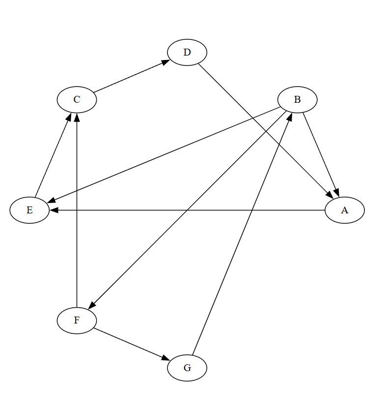
The reverse graph \(G^T\) reverses all edge directions, as shown below:

Let us walk through Kosaraju's algorithm:

Step 1: First DFS (computing finish times)

We perform DFS on the original graph \(G\) and record the finish time \(f[v]\) for each vertex.

Start Node	DFS Path	Finish Times f[v]
A	A -> E -> C -> D -> A	\(f[D]=6, f[C]=7, f[E]=8, f[A]=9\)
B	B -> F -> G -> B	\(f[G]=17, f[F]=18, f[B]=19\)

Assume we start from A, then from B, and check adjacency lists in the order A, B, C, D, E, F, G.

Finish times for all vertices:

Vertex	A	B	C	D	E	F	G
\(f[v]\)	9	19	7	6	8	18	17

---

Step 2: Sort vertices

Sort all vertices by their finish times \(f[v]\) in decreasing order to obtain a list \(L\).

Finish time f[v]	19	18	17	9	8	7	6
Vertex \(v\)	B	F	G	A	E	C	D

Sorted list \(L\): \([B, F, G, A, E, C, D]\)

---

Step 3: Construct the reverse graph \(G^T\)

Reverse all edge directions in the original graph \(G\) to obtain the reverse graph \(G^T\).

Edges of \(G^T\):

• A \(\leftarrow\) B, D
• E \(\leftarrow\) A, B
• F \(\leftarrow\) B
• D \(\leftarrow\) C
• C \(\leftarrow\) E, F
• G \(\leftarrow\) F
• B \(\leftarrow\) G

---

Step 4: Second DFS (finding SCCs)

Using the reverse-finish-time list \(L = [B, F, G, A, E, C, D]\) from Step 2, we perform DFS on the reverse graph \(G^T\) in that order. Each time a new traversal starts from an unvisited vertex, the set of discovered vertices constitutes one SCC.

1. Process vertex \(\text{B}\): B is the first unvisited vertex in list \(L\). We start DFS from it. In \(G^T\), the traversal path is \(\text{B} \to \text{G} \to \text{F} \to \text{B}\). All vertices reached in this DFS form the first SCC: \(\{\text{B}, \text{F}, \text{G}\}\). After this traversal, B, F, and G are marked as visited.
2. Process vertices \(\text{F}\) and \(\text{G}\): Although F and G follow B in list \(L\), they have already been marked as visited (belonging to the previous SCC), so they are skipped.
3. Process vertex \(\text{A}\): A is the next unvisited vertex in \(L\). We start a second DFS from A. A's neighbors include B and D; since B is already visited, we only follow D. The traversal path is \(\text{A} \to \text{D} \to \text{C} \to \text{E} \to \text{A}\). During traversal, although A or E in \(G^T\) may point to the already-visited B, DFS does not continue along visited nodes. The vertices discovered in this traversal form the second SCC: \(\{\text{A}, \text{C}, \text{D}, \text{E}\}\). We mark A, C, D, and E as visited.
4. Process vertices \(\text{E}, \text{C}, \text{D}\): The remaining vertices in \(L\) have all been marked as visited, so they are skipped.

All vertices have now been processed. The strongly connected components found are \(\{\text{B}, \text{F}, \text{G}\}\) and \(\{\text{A}, \text{C}, \text{D}, \text{E}\}\), which is correct.

Tarjan's Algorithm

SCC Contraction

Within an SCC, you can visit any other node in that SCC and return to the starting point. From an algorithmic perspective, an SCC is a "whole" -- you can traverse paths to collect all node attributes within the SCC (e.g., coins in the classic Coin Collector problem).

By compressing each individual SCC into a new single node (commonly called an SCC node), and setting the new node's weight as the sum of all original node weights, we perform an SCC contraction, also known as graph condensation.

Changes after SCC contraction:

• Node transformation: Each SCC in the original graph \(G\) is compressed into a single node in the new graph \(G'\) (commonly called a super node or SCC node).
• Node weights: The weight of the new node \(C_i\) equals the sum of all original node attributes it contains (e.g., the total number of coins).
• Edge transformation: If the original graph \(G\) has an edge \(u \to v\), where \(u\) belongs to SCC \(C_A\) and \(v\) belongs to SCC \(C_B\): if \(C_A = C_B\), this edge is ignored in \(G'\) (as it is internal to the SCC); if \(C_A \neq C_B\), a new edge \(C_A \to C_B\) is added in \(G'\).

The condensed graph \(G'\) has a crucial property:

The condensation graph \(G'\) is always a directed acyclic graph (DAG).

Taking the maximum-sum path problem as an example (i.e., the Coin Collector example below), the problem can be decomposed into three clear steps:

Phase	Objective	Algorithm	Complexity
I. SCC Computation	Find all SCCs in the original graph \(G\) and compute their total weights	Kosaraju or Tarjan algorithm	\(O(N+M)\)
II. DAG Construction	Build the condensation graph \(G'\) based on inter-SCC connections	Traverse all edges of \(G\)	\(O(N+M)\)
III. Path Optimization	Find the maximum-sum path on the weighted DAG \(G'\)	Topological sort + DP	\(O(N_{SCC} + M_{DAG}) \le O(N+M)\)

Whether using Kosaraju's or Tarjan's algorithm, the time complexity for SCC contraction is \(O(N+M)\).

Through SCC contraction, we can perform a quasi-topological sort on cyclic directed graphs -- essentially converting them to standard DAGs first, then applying topological sort.

Biconnected Components (BCC)

Biconnected components apply to undirected graphs.

Biconnected Components (BCC) refer to fault-tolerant substructures in undirected graphs. In simple terms, within a BCC, at least two elements must be destroyed to disconnect it. Based on whether vertices or edges are destroyed, BCCs are classified into two types:

• Edge-Biconnected Component (e-BCC)
• Vertex-Biconnected Component (v-BCC)

v-BCC is slightly more complex than e-BCC, but it is also the more commonly used definition. In general, when "biconnected component" is mentioned without further specification, it typically refers to v-BCC.

e-BCC

An undirected graph (or subgraph) is edge-biconnected if it:

1. Is connected.
2. Contains no bridge (bridge-free).
3. That is: removing any single edge leaves the graph connected.

An edge-biconnected component (e-BCC) is a maximal edge-biconnected subgraph of an undirected graph. "Maximal" means you cannot add any more nodes or edges to the subgraph without introducing a bridge, which would violate the edge-biconnected property.

Properties and structure of e-BCC:

• Contraction: If we treat each edge-biconnected component as a "super node" and the original bridges as connecting edges, the original graph becomes a tree (or forest).
• Equivalent condition: By Menger's Theorem, a graph is edge-biconnected if and only if there exist at least two edge-disjoint paths between any two vertices.

Finding e-BCCs typically uses the Tarjan Cut algorithm:

Use Tarjan Cut to find all bridges, then perform another DFS/BFS: any vertices reachable without crossing a bridge belong to the same e-BCC.

v-BCC

When "biconnected component" is mentioned without qualification, it typically refers to v-BCC.

An undirected graph (or subgraph) is vertex-biconnected if it:

1. Is connected.
2. Contains no cut vertex.
3. That is: removing any single vertex leaves the graph connected.

A vertex-biconnected component (v-BCC) is a maximal vertex-biconnected subgraph of an undirected graph.

Note that edge-biconnectedness is transitive: if x and y are edge-biconnected, and y and z are edge-biconnected, then x and z are edge-biconnected. However, vertex-biconnectedness is not transitive. The counterexample below shows that A and B are vertex-biconnected, B and C are vertex-biconnected, but A and C are not vertex-biconnected.

In v-BCC, a cut vertex can belong to multiple vertex-biconnected components simultaneously.

• Intuition: Imagine two iron rings linked together. The linking point is the cut vertex. The left ring is one v-BCC, the right ring is another v-BCC, and the middle point is shared by both.

Edge membership: Every edge in the graph belongs to exactly one vertex-biconnected component.

Since cut vertices belong to multiple components, we cannot simply compress components into single nodes as with e-BCCs. Instead, we need to construct a special tree called the Block-Cut Tree.

Unlike e-BCC, v-BCC is not transitive, which means we cannot simply find cut vertices and remove them. One must always remember:

A cut vertex is itself part of the v-BCC.

Therefore, after finding cut vertices with the Tarjan Cut algorithm, we cannot simply delete them. Instead, the cut vertex must be duplicated and assigned to each component it belongs to. Hence, finding v-BCCs requires a stack.

Block-Cut Tree

The Block-Cut Tree is specifically designed for vertex-biconnected components (v-BCC). It transforms the complex entanglement in the original graph into a clear tree-structured relationship.

The idea behind the Block-Cut Tree is: Since a cut vertex belongs to both component A and component B, instead of merging vertices, we create virtual nodes to represent the components. In the Block-Cut Tree, each original vertex corresponds to a round node, and each v-BCC corresponds to a square node.

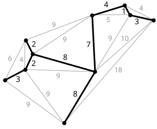
Minimum Spanning Tree (MST)

A Minimum Spanning Tree (MST) is a spanning tree of a connected weighted undirected graph with the minimum total edge weight. As shown below:

By the properties of trees, we know an MST must:

• Include all n vertices of the original graph
• Have exactly n-1 edges
• Be connected
• Have the minimum total weight among all possible spanning trees of the graph

Core Properties of MST

MSTs have several critically important properties that should be memorized:

1. Cut property: For any cut in the graph, if one crossing edge is strictly lighter than all others, that edge must be in the MST.
2. Cycle property: In any cycle, if one edge is strictly heavier than all others, that edge will not be in the MST.
3. If there exists an edge in the graph that is strictly lighter than all other edges, that edge must be in the MST.
4. If all edge weights in the graph are distinct, then the MST is unique.

Cut Lemma

The Cut Lemma, also commonly called the Cut Property or Cut Theorem, is the foundation for the correctness of Minimum Spanning Tree (MST) algorithms such as Prim's and Kruskal's.

The Cut Lemma states:

Given a connected, weighted graph \(G = (V, E)\), let \((S, T)\) be a cut of \(G\). If edge \(e=(u, v)\) is the minimum-weight edge in the cut set \(\delta(S)\) (i.e., \(w(e) \le w(f)\) for all \(f \in \delta(S)\)), then edge \(e\) must belong to some minimum spanning tree of \(G\).

The Cut Lemma guarantees that in graph \(G=(V, E)\), if an edge is the lightest among all edges crossing a cut, then it must belong to some MST of \(G\).

Minimax Property

The maximum edge refers to the heaviest edge on a path. Minimax means minimizing the heaviest edge on a path.

MST automatically satisfies the minimax property:

In any graph, the path between any two vertices in the MST is the one with the smallest maximum edge among all possible paths.

Alternatively stated:

The MST has the minimum total weight among all bottleneck spanning trees.

A Bottleneck Spanning Tree is a spanning tree whose maximum edge weight is minimized. An MST is always a bottleneck spanning tree, but a bottleneck spanning tree is not necessarily an MST.

The reason MST is always a bottleneck spanning tree is that MST:

• Selects small edges first
• Avoids using large edges whenever possible
• Never jumps to a larger edge when connectivity can be achieved without one

Therefore, the maximum edge in an MST is already as small as possible, and the MST is necessarily a bottleneck-optimal spanning tree.

Minimax is a very important property of MSTs and can solve numerous real-world problems, such as:

• Finding the path that minimizes maximum latency
• Finding the path that minimizes maximum danger/difficulty, e.g., mountain climbing routes
• Finding the minimum bottleneck path between two points
• Network bandwidth optimization: finding the route that minimizes the maximum latency bottleneck

The minimum bottleneck path mentioned above refers to the path between two points, among all possible paths, that minimizes the weight of the worst (heaviest) edge. The path between two points in the MST is naturally the minimum bottleneck path.

Here, the minimum bottleneck is essentially about minimizing the maximum edge. Think of edges as network latency or traffic congestion: the biggest bottleneck in a network is the segment with the highest latency or worst congestion. The minimum bottleneck route tries to ensure the most congested segment is as uncongested as possible -- that is, minimax.

Prim's Algorithm (Growing a Tree)

Prim's algorithm grows a tree from a single node to N nodes. In each "growth" round, a new node and edge are added. Throughout the process, the tree remains acyclic and connected. Note that Prim's algorithm only records each node's shortest distance to the MST.

The core idea of standard Prim's algorithm is greedy: starting from one vertex, it always adds the nearest node to the current spanning tree. The main steps are:

• Initialize a min-heap to store all vertices. Set the starting vertex \(r\)'s key (distance) to 0 and all other vertices' key to infinity (\(\infty\)).
• Main loop -- while the min-heap is not empty:
  • Extract-Min: Remove the vertex \(u\) with the smallest key and add it to the MST.
  • Relax: Traverse all neighbors \(v\) of \(u\). If \(v\) is still in the priority queue and the edge weight \(w(u, v)\) is less than \(v\)'s current key, update \(v.key = w(u, v)\) and set \(v\)'s parent to \(u\). This step requires a Decrease-Key operation.

Clearly, if the graph has V vertices, Prim's requires V iterations.

Time complexity analysis of Prim's algorithm:

• Initialization: Building the heap requires \(O(V)\)
• The outer loop runs \(V\) times (each vertex is dequeued once via Extract-Min). Extracting the minimum from a min-heap (with removal) costs \(O(\log V)\), totaling \(O(V\log V)\).
• Relax: The inner loop traverses all edges. For each edge, a Decrease-Key may be performed. Modifying a value and sifting up in a min-heap costs \(O(\log V)\), with at most \(E\) occurrences, totaling \(E \log V\).

Therefore, the total time complexity is:

\[ O(V \log V + E \log V) = O((V+E) \log V) \]

For connected graphs, typically \(E \ge V-1\), so this is usually simplified to \(O(E \log V)\).

Note that using a Fibonacci heap, Prim's time complexity can be reduced to \(O(E + V \log V)\). However, whether the Fibonacci heap yields a practical speedup depends on the relationship between \(E\) and \(V\). For dense graphs where \(E \approx V^2\), the Fibonacci heap is faster. But Fibonacci heaps are very complex to implement, so in practice, Prim's algorithm typically uses a standard min-heap.

Bucket Sort Optimization

Consider this special case: edge weights are integers in the set \(\{1, 2, \dots, k\}\), where \(k = O(1)\) (i.e., \(k\) is a small constant).

We already know that Prim's bottleneck lies in the \(O(\log V)\) cost of extracting the minimum from the heap and the \(O(\log V)\) cost of sifting up during Decrease-Key. For cases satisfying the special condition above -- where the range of weights is very small (similar to exam scores or age ranges) -- we can replace comparison-based sorting structures (heaps) with a bucket sort or counting sort approach.

Data structure replacement:

• No longer use a binary heap.
• Use an array of size \(k+1\) instead. Array indices \(0, 1, \dots, k\) represent possible edge weights.
  • Note that the bucket indices themselves represent edge weights and are naturally ordered from small to large. Thus, we simply find the first non-empty bucket starting from index 0, and it must contain the minimum value.
• Each array position stores a doubly linked list containing vertices with that key value.
  • Why a doubly linked list? Because we need \(O(1)\) deletion from the middle of the list (for Decrease-Key). For example, if a node's weight drops from 10 to 2, we move it from bucket 10 to bucket 2. Since we have stored the node pointer for vertex v in a Pos array, the adjustment is fast -- something that list, set, or other data structures cannot achieve.

Here is the algorithm flow for this special case:

Input: Connected graph \(G=(V, E)\), edge weights \(w(u, v) \in \{1, 2, \dots, k\}\), starting vertex \(r\).

Data structures:

1. Buckets: Array B of size \(k+1\), where B[i] is a doubly linked list.
2. Key array: key[v] stores vertex \(v\)'s minimum distance to the MST, initialized to \(\infty\).
3. InMST array: Boolean flags indicating whether a vertex has been processed.
4. Pos array: pos[v] stores a pointer to vertex \(v\)'s node in the doubly linked list (for \(O(1)\) deletion).

Algorithm steps:

1. Initialization:

• Set all vertices' key to \(\infty\) and parent to NULL.
• Set key[r] = 0 for the starting vertex.
• Insert \(r\) into linked list B[0] and update pos[r].

1. Main loop:

• Define variable idx = 0 (current minimum bucket index being scanned).
• While the MST does not include all vertices:
  • a. Extract-Min (find minimum vertex):
    • While B[idx] is empty, execute idx = idx + 1. (Find the first non-empty bucket.)
    • Remove vertex \(u\) from the head of B[idx].
    • Mark u as InMST = true.
  • b. Relax (relax adjacent edges):
  • For each neighbor \(v\) of \(u\) with edge weight \(w\):
    • If \(v\) is not in the MST and \(w < key[v]\):
      • Step i (remove old value): If key[v] is not \(\infty\), use the pos[v] pointer to remove \(v\) from bucket B[key[v]] (\(O(1)\) operation).
      • Step ii (update data): Update key[v] = w, parent[v] = u.
      • Step iii (insert new value): Insert \(v\) at the head of bucket B[w].
      • Step iv (update pointer): Update pos[v] to point to the new position.
      • Optimization detail: If \(w < idx\), reset idx = w (not required but speeds up searching).

1. Termination: Output the MST defined by the parent array.

Time complexity:

• Extract-Min:
  • Operation: Scan from index 0 to find the first non-empty list. Remove the head element.
  • Cost: Since \(k\) is a constant \(O(1)\), scanning the array takes constant time. Removing from the list head is also \(O(1)\). So Extract-Min is \(O(1)\).
• Decrease-Key:
  • Operation: When reducing vertex \(v\)'s weight from old_w to new_w:
    1. Find \(v\) in the doubly linked list at index old_w and remove it (\(O(1)\), given we maintain node pointers).
    2. Insert \(v\) at the head of the list at index new_w (\(O(1)\)).
  • Cost: The entire process involves only linked list pointer operations, costing \(O(1)\).

Total time complexity:

• Extract-Min: Executed \(V\) times, each \(O(1)\) \(\rightarrow\) total \(O(V)\).
• Decrease-Key: Executed \(E\) times, each \(O(1)\) \(\rightarrow\) total \(O(E)\).
• Total: \(O(V + E)\).

---

Let us look at a concrete application. Suppose you are building a tile-based game or city planning simulator, where you need to lay the cheapest oil pipeline or power grid (a minimum spanning tree problem).

The map is divided into an \(N \times M\) grid. Each tile is a node. The graph is very large (e.g., a \(1000 \times 1000\) map with 1 million nodes). Each tile connects only to its up/down/left/right neighbors (a grid graph).

Terrain determines the cost of laying pipelines. There are very few terrain types. The costs are defined as:

• Grass: cost = 1
• Forest: cost = 2
• Sand: cost = 3
• Shallow Water: cost = 4
• Rock: cost = 5

Note: There are no costs like 1.54 or 3.99 -- costs strictly belong to the integer set \(\{1, 2, 3, 4, 5\}\). Here \(k=5\).

This scenario has two key characteristics:

• Massive data: For a large high-resolution map, vertex count \(V\) can reach millions, with edge count \(E \approx 4V\).
• Tiny weight range: \(k\) is only 5.

A rough comparison of the two Prim variants:

• Standard Prim (\(E \log V\)): \(4{,}000{,}000 \times \log_2(1{,}000{,}000) \approx 4{,}000{,}000 \times 20 = 80{,}000{,}000\) operations.
• Optimized Prim (\(E + V\)): \(4{,}000{,}000 + 1{,}000{,}000 = 5{,}000{,}000\) operations.

The optimized algorithm is roughly 16 times faster, which is a huge advantage in real-time rendering or game loading.

Fibonacci Heap Optimization

As mentioned earlier, the Fibonacci heap can theoretically provide optimization but is complex to implement, so it is rarely used in practice (unless specifically needed).

Using a binary heap:

\[ \text{Total cost} \approx \underbrace{E \times \log V}_{\text{processing edges}} + \underbrace{V \times \log V}_{\text{processing vertices}} \]

• Pain point: Each edge processed (relaxation) incurs a \(\log V\) cost.

Using a Fibonacci heap:

\[ \text{Total cost} \approx \underbrace{E \times 1}_{\text{processing edges}} + \underbrace{V \times \log V}_{\text{processing vertices}} \]

• Breakthrough: Processing each edge now costs only a constant \(1\) (amortized).

With a Fibonacci heap, edge processing becomes extremely cheap, and the algorithm bottleneck shifts from edges back to vertices (\(V \log V\)). In most practical connected graphs, the number of edges exceeds the number of vertices, so shifting the bottleneck from edges to vertices is meaningful.

Kruskal's Algorithm (Forest Merging)

Kruskal's basic idea is to maintain a forest and, in each iteration, find an eligible edge to connect two trees. When only one tree remains in the forest, that tree is the MST.

Clearly, if the graph has E edges, Kruskal's iterates at most E times.

Treating every vertex in the graph as an individual tree, the algorithm outline is:

Kruskal's Algorithm

Use a min-heap (priority queue) to store all edges and their weights
Set T records all selected edges, initially empty

Loop (until T has graph's vertex count - 1 edges):
    Extract the minimum edge from the min-heap:
        If the two endpoints belong to different trees, add the edge to T and merge the two trees

Kruskal's time complexity is \(O(E \lg V)\). (Note: a union-find data structure must be used; see the union-find section.)

Disjoint Set Union (DSU)

Union-Find is a data structure for managing disjoint sets (Disjoint Set Union, DSU).

The core operations of union-find include:

• MakeSet: Create an independent set for each element
• Union: Merge the sets containing two elements
• Find: Query the representative of the set containing a given element

The main applications of union-find include:

• Detecting cycles in a graph
• Checking whether two nodes belong to the same tree in Prim's algorithm

Note: Union-find is suitable for merging and querying, but not for splitting sets.

---

Path compression and union by rank dramatically improve union-find's time complexity:

Optimization Strategy	FIND Time	UNION Time	Notes
No optimization	O(n)	O(n)	Chain-shaped tree, worst case
Path compression	O(α(n))	O(α(n))	Tree flattens but may be unbalanced
Union by rank	O(log n)	O(log n)	Height is bounded
Path compression + Union by rank	O(α(n)) ≈ O(1)	O(α(n)) ≈ O(1)	Strongest, unbeatable

In general, "union-find" implicitly refers to the version optimized with both path compression and union by rank.

The \(\alpha(n)\) in the table above is the Inverse Ackermann Function, which grows extremely slowly -- even with all atoms in the universe, its value would not exceed 4. Therefore, in engineering practice, optimized union-find operations are effectively considered \(O(1)\).

---

Parent array

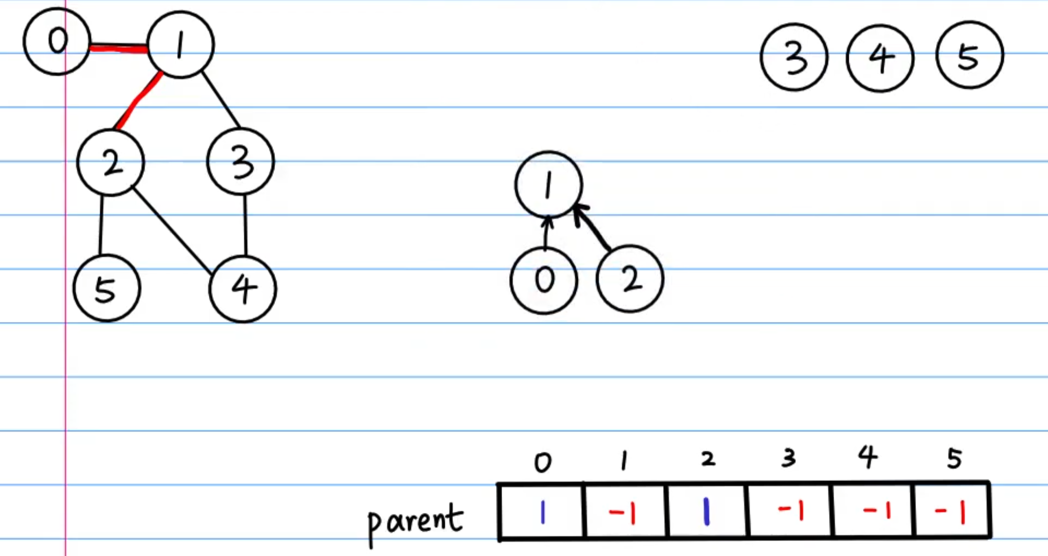
We use an array called parent to record each node's parent.

For non-integer nodes, a dictionary can serve as the mapping: map = {node: index}

The parent array is the core of union-find. Any node can follow the parent array upward until reaching the root (whose value is typically set to -1).

In other words, the FIND operation in union-find essentially locates the root of the tree containing a given node. If two nodes share the same root, i.e., find(x) == find(y), then x and y are in the same set.

Similarly, the UNION operation essentially makes the root of one set point to the root of another set. For example:

Root of set A = rootA
Root of set B = rootB

To merge sets A and B, simply set parent[rootA] = rootB.

Important: you must not directly set x's parent to y. You must use the find operation to locate the roots first. Only set roots can represent entire sets. Setting an intermediate node's parent to another node would sever the set tree, corrupting the entire structure.

---

Path Compression

Path compression is the most critical optimization in union-find:

During FIND, while traversing to the root, make all nodes on the path point directly to the root.

Path compression dramatically reduces tree height, so subsequent lookups for these nodes reach the root in a single step, greatly improving performance.

The path compression code is very concise:

def find(x):
    if parent[x] != x:
        parent[x] = find(parent[x])   # ★ 路径压缩
    return parent[x]

.

---

Union by Rank

Union by rank means that during union, the shorter tree (smaller rank) is always attached to the taller tree (larger rank). This prevents unnecessary growth in tree height. Here, "rank" approximately represents tree height. A variant called "Union by Size" achieves a similar effect.

Implementations

Legacy Version

This section introduces the legacy teaching version (also called the classic version). Note that this version only provides insight into how early researchers constructed union-find, but nobody uses this method in modern engineering practice. The differences between the legacy and modern approaches are:

• Legacy version: Linked list + weighted union (never used in engineering practice)
• Modern approach: Tree structure + path compression + union by rank (used in engineering practice)

The legacy version is presented here mainly to address the teaching requirements of some schools and courses. In the early days of computer science, the linked list approach did exist briefly. Here is a rough historical timeline of union-find in practice:

1. Ancient version at the dawn of computing: Naive tree structure
2. Legacy version from early computing: Linked list + weighted union
3. Modern approach (established 1975): Tree structure + path compression + union by rank

In 1975, Tarjan proved in the paper "Efficiency of a Good But Not Linear Set Union Algorithm" that path compression combined with union by rank achieves \(O(\alpha(n))\), which is near-optimal. This is why, a full 50 years later, it is frustrating when courses still teach the linked list approach.

Let us examine how the legacy version uses linked lists to implement union-find. In the legacy version, a set is a singly linked list. The set object (or dummy head) is a special management object; each set has one. It contains three key fields:

• Head: Points to the first element of the linked list
• Tail: Points to the last element (for convenient tail appending)
• Size: Records the number of elements in the linked list (for weighted union)

Element nodes contain:

• val: The data itself
• Next: Points to the next node
• Rep: Points to the set object

The three core operations work as follows:

1. MAKE-SET(x)
   • Create a new set object with Head and Tail pointing to x, Size = 1
   • x's Rep points to itself
   • Complexity: O(1)
2. FIND-SET(x)
   • Take node x, follow Rep to find the set object, return the set object's Head
   • Complexity: O(1)
3. UNION(x, y)
   • Find x's set S_x and y's set S_y
   • Compare the sizes of S_x and S_y; append the smaller one to the larger one:
     • S_x.Tail.next = S_y.Head
     • S_x.Tail = S_y.Tail
     • S_x.Size = S_x.Size + S_y.Size
   • Finally, update pointers: traverse every node in the smaller set S_y and change Rep to S_x

The most expensive step is updating pointers during UNION. If we do not check sizes and merge randomly, we might repeatedly merge a large set into a small one, forcing updates to all pointers in the large set. The worst-case single UNION is \(O(n)\).

However, we can use a smarter approach: weighted union. We only update the smaller set's member pointers. If an element \(k\)'s pointer is modified, it means its set was merged into a larger set. After merging, the new set is at least twice the size of the original (since large \(\ge\) small, so large + small \(\ge\) 2 * small). With \(n\) total elements, a set can double from size 1 to \(n\) at most \(\log_2 n\) times. This means any element's pointer is modified at most \(\log_2 n\) times:

• Total complexity: \(m\) operations cost \(O(m + n \log n)\).
• Amortized cost: On average, each UNION is \(O(\log n)\).

For the legacy version, just remember: UNION's amortized time complexity is O(log N). This is much slower than the modern approach's O(\(\alpha(N)\)). The reason Tarjan called the modern approach "not linear" is that although the inverse Ackermann function is practically near-linear, in the mathematical sense of infinity it does continue to grow. In other words, \(m \cdot \alpha(n)\) is not strictly linear \(m\). It is an extremely, extremely flat upward-curving line that is technically "super-linear."

Tarjan proved that the modern approach with path compression and union by rank has a worst-case upper bound of \(O(m \alpha(n))\), demonstrating how fast the algorithm is. Later, in 1989, Fredman and Saks proved in their paper "The cell probe complexity of dynamic data structures" that Tarjan's modern approach is the theoretical lower bound. In other words, no union-find algorithm can theoretically achieve true \(O(1)\) average time (i.e., total time \(O(m)\)), even with a quantum computer (in the classical data structure context).

Standard Union-Find

Having understood the core concepts above, let us look at the implementation of the standard union-find (the modern approach with path compression and union by rank). Note: mastery of the standard union-find is essential, as it is a frequently used data structure.

In competitive programming and high-performance scenarios, using arrays for the parent structure is the most common approach. In most graph theory and union-find problems, nodes are typically given as integers from 0 to n-1, or as coordinates in a 2D matrix (which can be converted to integer indices).

However, for non-integer nodes, using a dictionary is more convenient.

Standard union-find implementation:

class UnionFind:
    def __init__(self, n):
        self.parent = list(range(n))
        self.rank = [1] * n
        self.count = n  # 记录连通分量数量

    def find(self, p):
        if self.parent[p] != p:
            self.parent[p] = self.find(self.parent[p]) # 路径压缩
        return self.parent[p]

    def union(self, p, q):
        rootP = self.find(p)
        rootQ = self.find(q)
        if rootP == rootQ:
            return False

        # 按秩合并
        if self.rank[rootP] > self.rank[rootQ]:
            self.parent[rootQ] = rootP
        elif self.rank[rootP] < self.rank[rootQ]:
            self.parent[rootP] = rootQ
        else:
            self.parent[rootQ] = rootP
            self.rank[rootP] += 1

        self.count -= 1
        return True

If the input nodes are non-integer (e.g., "A", "B", "C"), we use a dict-based implementation:

class UnionFind:
    def __init__(self):
        self.parent = {} # 存储节点的父节点 {node: parent_node}
        self.rank = {} # 存储树的高度/秩 {node: rank_value}
        self.count = 0 # 记录连通分量的数量

    def add(self, x):
        # 添加新节点 x。如果 x 已经存在，则什么都不做。
        if x not in self.parent:
            self.parent[x] = x
            self.rank[x] = 1
            self.count += 1

    def find(self, p):
        # 查找 p 的根节点，并进行路径压缩。
        # 如果 p 不存在，可以选择报错或者自动添加（这里选择自动添加以增强鲁棒性）。
        if p not in self.parent:
            self.add(p)
            return p # 新加的节点，根就是自己

        # 路径压缩 (Path Compression)
        if self.parent[p] != p:
            self.parent[p] = self.find(self.parent[p])
        return self.parent[p]

    def union(self, p, q):
        # 合并 p 和 q 所在的集合。
        rootP = self.find(p)
        rootQ = self.find(q)

        if rootP == rootQ:
            return False

        # 按秩合并 (Union by Rank)
        if self.rank[rootP] > self.rank[rootQ]:
            self.parent[rootQ] = rootP
        elif self.rank[rootP] < self.rank[rootQ]:
            self.parent[rootP] = rootQ
        else:
            self.parent[rootQ] = rootP
            self.rank[rootP] += 1

        self.count -= 1
        return True

    def is_connected(self, p, q):
        return self.find(p) == self.find(q)

If the input is an adjacency list:

def solve_adjacency_list(n, adj):
    """
    :param n: 节点总数 (有些题目没给 n，可能需要先遍历 adj 计算节点数)
    :param adj: 邻接表，例如 {0: [1], 1: [0, 2], 2: [1]}
    """
    uf = UnionFind(n)

    for u in adj:
        for v in adj[u]:
            # 对每一条边进行合并
            # 并查集内部会处理重复合并（即 union(u, v) 和 union(v, u) 是一样的）
            uf.union(u, v)

    return uf.count

# --- 测试案例 ---
# 5个节点 (0-4)
# 0-1, 1-2 相连 (一组)
# 3-4 相连 (一组)
n_nodes = 5
adj_list = {
    0: [1],
    1: [0, 2],
    2: [1],
    3: [4],
    4: [3]
}

print(f"邻接表连通分量数: {solve_adjacency_list(n_nodes, adj_list)}") # 输出: 2

If the input is an adjacency matrix:

def solve_adjacency_matrix(matrix):
    n = len(matrix)
    uf = UnionFind(n)

    # 遍历矩阵
    for i in range(n):
        # j 从 i + 1 开始，只遍历右上三角，避免重复检查 (i, j) 和 (j, i)
        # 同时也跳过了 M[i][i] 这种自环
        for j in range(i + 1, n):
            if matrix[i][j] == 1:
                uf.union(i, j)

    return uf.count

# --- 测试案例 ---
# 3个节点的图：0和1相连，2单独
adj_matrix = [
    [1, 1, 0],
    [1, 1, 0],
    [0, 0, 1]
]
print(f"邻接矩阵连通分量数: {solve_adjacency_matrix(adj_matrix)}") # 输出: 2

.

Weighted Union-Find

The standard union-find only records "who is my root." A weighted union-find additionally maintains a value (weight) alongside the parent pointer, representing the "relationship between the current node and its parent":

Core idea: Treat nodes as vertices in a graph, where edge weights represent relationships. Through vector addition (or multiplication/XOR), we can compute the total distance from any node to its root.

During path compression: val[x_to_root] = val[x_to_parent] + val[parent_to_root].

During union: Use the vector triangle rule to calculate the weight of the edge that should connect the two roots.

Weighted union-find is best suited for problems involving transitive "numerical" or "binary" relationships.

Interval sums / difference constraints:

• Given \(A-B=3, B-C=2\), find \(A-C\).
• Here, the "weight" is a numerical difference.

Parity / group verification (LeetCode 886):

• A and B are in different groups, B and C are in different groups \(\rightarrow\) A and C are in the same group.
• Here, the "weight" is addition modulo 2 (\(1+1=0\)).

Ratio relationships (LeetCode 399):

• A is 2 times B, B is 3 times C \(\rightarrow\) A is 6 times C.
• Here, the "weight" is multiplication.

Extended-Domain Union-Find

When nodes can have multiple possible states (e.g., friend/enemy, type A/B/C) and we do not know the specific state, we create all possible identities for each node.

Core idea: Since we do not know whether \(i\) is friend or foe, we split \(i\) into two nodes: i_friend and i_enemy.

Logical connections:

• If "\(i\) and \(j\) are enemies," we connect (i_friend, j_enemy) and (i_enemy, j_friend).
• This means: if \(i\) is a friend, then \(j\) is an enemy; if \(i\) is an enemy, then \(j\) is a friend.
• This forms a logical implication graph.

Extended-domain union-find is best suited for non-numerical problems with finite states and mutual exclusion:

Friend/enemy relationships / gang problems:

• The enemy of my enemy is my friend.
• Split into: \(i_{self}\) (self), \(i_{enemy}\) (enemy).

Food chains / cyclic dominance:

• A eats B, B eats C, C eats A.
• Split into three domains: \(i_{self}, i_{eat}, i_{enemy}\).

Simple 2-SAT problems:

• Conditional selection problems: choosing A means you cannot choose B.

Single-Source Shortest Paths (SSSP)

Single-Source Shortest Paths (SSSP).

The main algorithms include (applicable to both directed and undirected graphs):

• BFS: For unweighted graphs, \(\Theta(V+E)\)
• Dijkstra: For weighted graphs with no negative edges, \(\Theta((V+E) \log V)\)
• Bellman-Ford: For weighted graphs, negative edges allowed, \(\Theta(VE)\)

SSSP encompasses the following core concepts:

• Optimal substructure
• Negative-weight edges
• Negative-weight cycles
• Shortest-path representation
• Relaxation

---

Optimal Substructure

Optimal substructure:

A subpath of a shortest path is itself a shortest path.

Proof sketch: Use a "cut-and-paste" proof by contradiction. If a subpath were not the shortest, we could replace it with a shorter subpath, making the total path weight smaller -- contradicting the premise that the original path is "shortest."

---

Negative-Weight Edges

• Negative-weight edges:
  • Some algorithms (e.g., Dijkstra) require all edge weights to be non-negative.
  • Some algorithms (e.g., Bellman-Ford) allow negative-weight edges.
• Bellman-Ford algorithm:
  • Can handle negative-weight edges.
  • Can detect whether a negative-weight cycle is reachable from the source. If one exists, it reports it; if not, it produces correct results.

---

Negative-Weight Cycles

Normally, since we seek shortest paths, we would avoid positive-weight cycles. But what about negative-weight cycles? If we enter a negative-weight cycle, we can loop infinitely, reducing the total weight each time -- Dijkstra would break down in this scenario, whereas Bellman-Ford can detect negative-weight cycles.

Since positive-weight cycles waste cost and negative-weight cycles cause infinite loops, a legitimate, finite shortest path must contain no cycles. Therefore, a shortest path contains at most \(|V|-1\) edges.

---

Shortest-Path Representation

• Shortest-path estimate (\(v.d\)):
  • For each vertex \(v\), maintain an attribute \(v.d\) that records an upper bound on the shortest-path weight from source \(s\) to \(v\).
  • Initialization: \(s.d = 0\), all other vertices set to \(\infty\).
• Predecessor (\(v.\pi\)):
  • Records the parent in the shortest-path tree. By reversing the predecessor chain, we can reconstruct the shortest path from \(s\) to \(v\).
• Shortest-path tree:
  • A directed subgraph \(G'=(V', E')\) rooted at \(s\).
  • Contains all vertices reachable from \(s\).
  • The unique simple path from \(s\) to any vertex \(v\) in the tree is a shortest path from \(s\) to \(v\) in \(G\).
  • Note: Shortest paths are not necessarily unique, so shortest-path trees are not necessarily unique either.

---

Relaxation

Relaxation is the core operation of many SSSP algorithms.

• Definition: Check whether going through edge \((u, v)\) yields a shorter path from \(s\) to \(v\).
• Operation: If \(v.d > u.d + w(u, v)\), then update \(v.d = u.d + w(u, v)\) and set \(v\)'s predecessor to \(u\) (i.e., \(v.\pi = u\)).

Algorithm differences:

• Dijkstra: Relaxes each edge only once (based on a greedy strategy).
• Bellman-Ford: Relaxes each edge \(|V|-1\) times.

---

The following properties are commonly used in graph theory proofs:

Property	Core Meaning (Informal)	Key Point
Triangle Inequality	Shortcuts are shorter	The direct distance between two points \(\le\) any detour distance. \(\delta(s,v) \le \delta(s,u) + w(u,v)\)
Upper-bound Property	Estimates only decrease	The maintained distance \(v.d\) starts at infinity and only decreases. It never drops below the true distance. Once it reaches the true value, it locks in.
No-path Property	Unreachable means infinity	If there is no physical path, the distance remains \(\infty\).
Convergence Property	Correct predecessor yields correct successor	If \(u\)'s distance is correct and we relax edge \((u,v)\), then \(v\)'s distance also becomes correct.
Path-relaxation Property	Correct order guarantees correct result	As long as edges are relaxed in path order, regardless of other interleaved operations, the final result is correct.
Predecessor-subgraph Property	Predecessors form a tree	After the algorithm terminates, connecting all predecessor (parent) pointers yields a tree rooted at the source, with no cycles.

These properties guarantee that relaxation ultimately produces correct answers.

BFS-Based Approaches

For unweighted graphs, BFS naturally solves SSSP because BFS expands layer by layer.

In unweighted graphs, the "shortest path" is defined as having the fewest edges.

• Layer-by-layer expansion: BFS expands from the source, layer by layer.
  • Layer 0: the source.
  • Layer 1: all neighbors of the source (distance 1).
  • Layer 2: neighbors of neighbors (distance 2).
• Guaranteed shortest: Because BFS advances by layers, the first time a node \(v\) is visited, the path taken is guaranteed to have the fewest edges from the source to \(v\). No shorter path exists, or the node would have been visited in an earlier layer.

For a graph with \(V\) vertices and \(E\) edges:

• BFS complexity: \(O(V + E)\)
• This is linear and theoretically optimal for shortest path finding.

Bidirectional BFS

If the goal is to find the shortest path between a known source and destination (rather than from the source to all vertices), bidirectional BFS is faster.

• Principle: Simultaneously run BFS from both the source and destination until the two search frontiers meet.
• Advantage: Although the asymptotic complexity class remains the same, the search space (number of visited nodes) is typically significantly reduced (from \(b^d\) to \(2 \times b^{d/2}\)).

0-1 BFS

If the edge weights are not all 1, but only 0 and 1:

• Standard BFS does not work.
• Dijkstra works but is somewhat slower.

Best choice: Use a BFS with a deque (double-ended queue). Edges with weight 0 are added to the front; edges with weight 1 are added to the back. The complexity remains \(O(V+E)\).

Note that 0-1 BFS is specifically designed for SSSP problems with edge weights of only 0 or 1. It is essentially a specialization of Dijkstra, but since its code closely resembles BFS, it is conventionally called 0-1 BFS.

Core idea:

• Weight 0 edges: add to the front of the deque, processed with higher priority
• Weight 1 edges: add to the back of the deque, processed in normal order

This mechanism ensures that the element dequeued from the front always has the current shortest distance (similar to Dijkstra always popping the minimum-distance vertex).

Dijkstra-Based Approaches

Dijkstra's algorithm is the most classic algorithm in graph theory and the standard method for solving weighted SSSP problems. While BFS expands layer by layer, Dijkstra upgrades this idea: always process the cheapest node first.

Note that Dijkstra is an SSSP algorithm, so the dist values stored in its data structures represent the distance from the source to each vertex.

Dijkstra's core idea is greedy + relaxation:

• Greedy: Always extract the vertex with the currently known shortest distance (i.e., the minimum in the min-heap)
• Relaxation: Compare each neighbor's recorded distance with the newly computed distance

Using a min-heap, Dijkstra's algorithm:

• Extract-min: performed once per vertex, each costing O(log V) (heap height), totaling O(V log V)
• Decrease-key: each insert or update costs O(log E), occurring at most E times, totaling O(E log E)

Since \(E \le V^2\), we have \(\log E \le \log(V^2) = 2 \log V\). Therefore \(O(\log E)\) and \(O(\log V)\) are the same order.

Total complexity: \(O(V \log V + E \log V) = \mathbf{O((V+E) \log V)}\)

For the vast majority of algorithm problems and practical applications, graphs are sparse with E and V on the same order, i.e., \(E \ll V^2\). Also, Dijkstra's main bottleneck is the inner loop (decrease-key), which is triggered per edge. So it is typically simplified to: \(\mathbf{O(E \log V)}\)

Dial's Algorithm

When all edge weights are small positive integers, buckets can replace the heap, reducing Dijkstra's time complexity from \(O(E + V \log V)\) to theoretically linear time \(O(E + V)\).

Bellman-Ford-Based Approaches

Key points:

• Simple, but inefficient
• Can handle negative-weight edges and negative-weight cycles

Consider the diagram below. Dijkstra would lock in A->C as 3 and never update this path. However, the better route is A->B->C with a total cost of 2. In such cases, Bellman-Ford is needed.

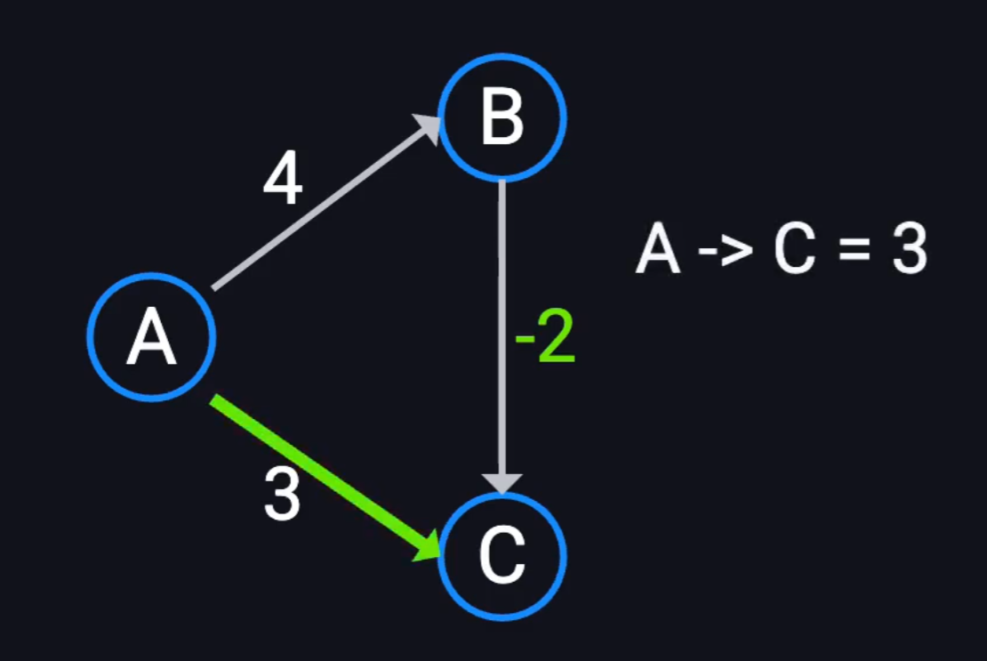
The core idea of Bellman-Ford is:

Repeatedly attempt to update all edges until all possible shortest paths have been found.

Here is the algorithm and a detailed walkthrough:

BELLMAN-FORD Algorithm

Initialize distances: (distance means from source to that vertex)
    Set source to 0, all other vertices to infinity
    Set all predecessors to null

Perform V-1 rounds of relaxation: (loop count = max possible path edges, typically V-1)
    Traverse all edges:
        For edge (u, v)
        Compute u.d + edge
        IF u.d + edge < v.d:
            v.d = u.d + edge
            v.predecessor = u
    If no vertex's distance was updated in this round, the result has converged; terminate early

If relaxation ran the full V-1 rounds, perform one additional round:
    Traverse all edges and relax
    If any vertex is updated:
        A negative-weight cycle exists; no shortest path is defined

After all vertex values converge, we have found shortest paths from the source to all vertices

As shown above, the outer loop runs V times and the inner loop runs E times, giving a time complexity of \(V \times E\).

---

Let us walk through an example of the Bellman-Ford algorithm.

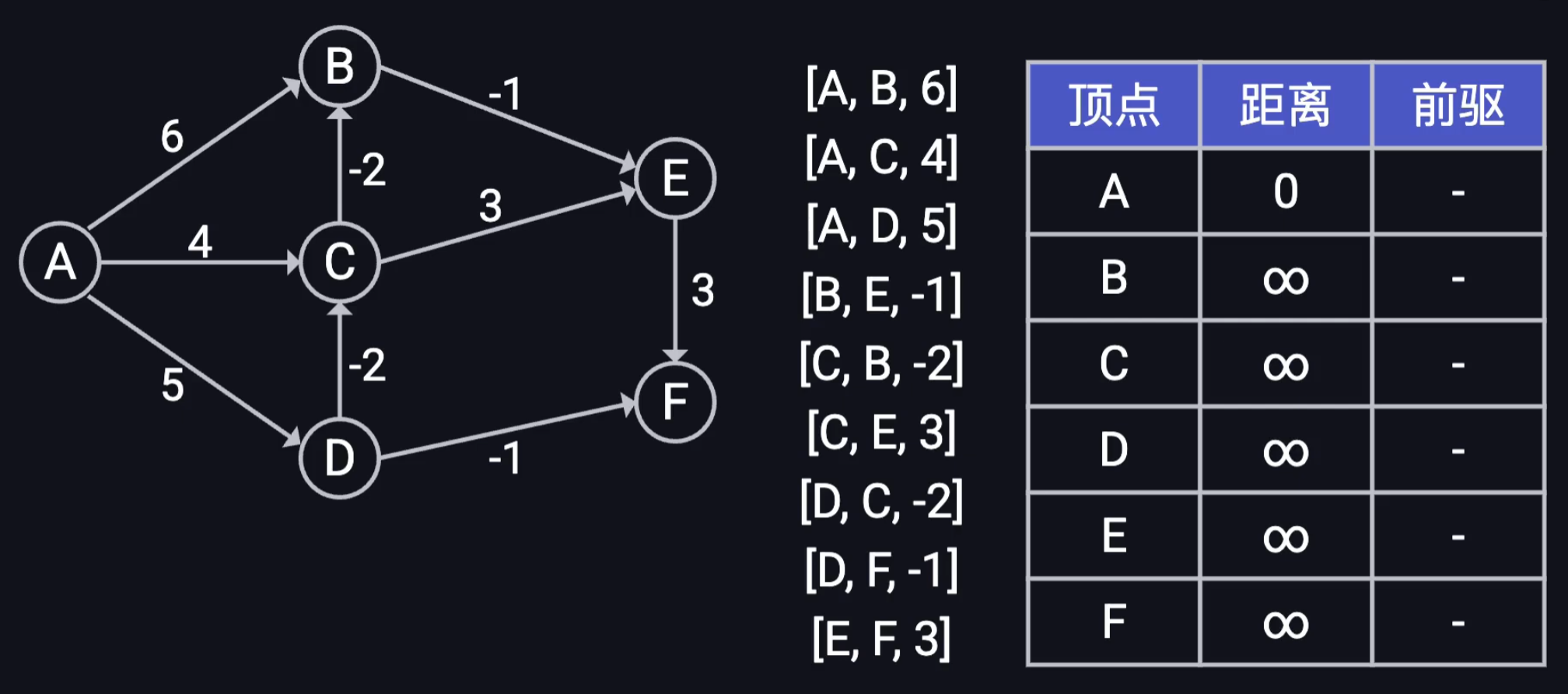
Note: The example walkthrough and images are from YouTube: Bobo Micro-lectures.

The graph has 6 vertices, so we need to perform 5 rounds of relaxation on every edge.

We initialize all vertices, choose A as the source, and record all edges.

The distance in the table means the distance from source A to that vertex; A's distance is always 0.

Round 1

After the first round of relaxation, all shortest paths reachable in exactly one step are guaranteed to be found.

...

Round 4

After the fourth round, traversing all edges reveals no new updates. The result has converged, so we can skip round 5 and also skip the extra V-th round of relaxation.

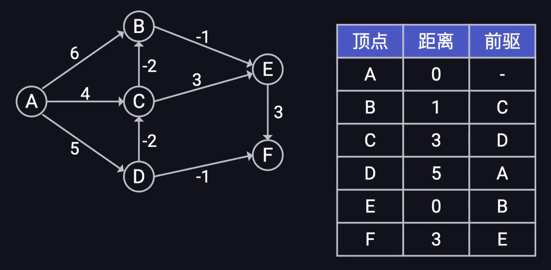
We can use predecessors to reconstruct the specific path from A to any other vertex.

Note that Bellman-Ford is an SSSP algorithm. In the example above, we computed with A as the center, so the results apply only to A. We cannot use this table to compute distances between other pairs unless they happen to lie on a path from A to another vertex, in which case the optimal substructure property allows us to extract that subpath.

SPFA Algorithm

SPFA stands for Shortest Path Faster Algorithm. It is internationally recognized as Bellman-Ford with queue optimization. This algorithm performs well on random sparse graphs and handles graphs with negative edge weights. However, SPFA's worst-case time complexity is the same as Bellman-Ford, so for graphs without negative edges, heap-optimized Dijkstra may outperform SPFA.

SPFA's basic idea is the same as Bellman-Ford: each node serves as a candidate for relaxing its neighbors. However, unlike Bellman-Ford, SPFA does not blindly attempt all nodes. Instead, it maintains a queue of candidate nodes and only enqueues nodes that have been relaxed. The process repeats until no more nodes can be relaxed.

Difference Constraint Systems

For example: A robot executing an action sequence where "action 2 must occur within [2s, 5s] after action 1."

• \(t_2 - t_1 \geq 2\)
• \(t_2 - t_1 \leq 5\)
• This is called a Simple Temporal Network (STN), whose core solving algorithm is based on Bellman-Ford or Floyd-Warshall for difference constraint solving.

This concept rarely appears in interviews or LeetCode. However, in practical applications, difference constraint systems are an important method for solving scheduling, layout, and time planning "constraint satisfaction problems." We will explore this topic further if needed.

---

All-Pairs Shortest Paths (APSP)

All-Pairs Shortest Paths (APSP).

We can certainly use SSSP to solve APSP -- for example, running Dijkstra or Bellman-Ford from every vertex. However, both approaches have inherent limitations for APSP:

• Running Dijkstra from every vertex has acceptable time complexity but cannot handle negative-weight edges.
• Bellman-Ford can handle negative-weight edges but has unacceptable time complexity.

Therefore, we need a dedicated all-pairs shortest path algorithm: Floyd-Warshall.

Note that for graphs with only positive edge weights, Dijkstra is typically faster than Floyd-Warshall.

Floyd-Warshall

Floyd-Warshall is essentially dynamic programming. We define a parameter k representing the set of allowed intermediate vertices. \(k\) does not refer to "one specific intermediate vertex" but rather "the range of the allowed set of intermediate vertices." \(DP[k][i][j]\) represents "the shortest path from \(i\) to \(j\) using only vertices numbered \(1 \dots k\) as intermediaries."

For efficient traversal, we typically maintain two matrices:

• Adjacency matrix recording shortest distances
• Next-hop matrix recording the next vertex on the path

State transition equation:

\[ dist[i][j] = \min(dist[i][j], \quad dist[i][k] + dist[k][j]) \]

Variable meanings:

• \(i\): source.
• \(j\): destination.
• \(k\) (most critical): the set of currently allowed intermediate vertices (\(1 \dots k\)).

If you only need the shortest distance (not the actual path), the next-hop matrix is not needed. Recording next-hop allows path reconstruction. For example, next[i][j] = 10 means the first hop from i to j is 10; then look up next[10][j], and so on until reaching next[j][j].

Floyd-Warshall works on graphs with negative-weight edges. Additionally, after traversal, negative-weight cycle detection can be performed by adding a simple check after the triple loop:

has_negative_cycle = False

for i in range(n):
    if dist[i][i] < 0:
        has_negative_cycle = True
        break

This means: if any \(dist[i][i] < 0\), the graph contains a negative-weight cycle. This is because at the start of the algorithm, the distance from any vertex to itself is set to 0. Suppose there is a cycle \(A \to B \to C \to A\) with total edge weight \(-10\). During the algorithm, when attempting to update the distance of \(A \to A\), the negative value will cause an incorrect update, thereby detecting the negative-weight cycle.

---

Let us work through an example:

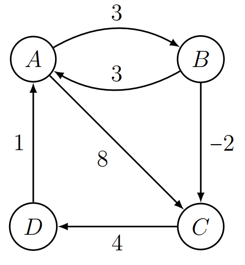
Using the above graph, let us see how Floyd-Warshall executes.

Imagine the nodes as airports, edges as routes, and weights as flight times. Floyd-Warshall's core idea is to progressively unlock intermediate stops:

• First, consider no intermediate cities at all, denoted \(D^{(0)}\).
• Then, consider A as an allowed intermediate, denoted \(D^{(1)}\).
• Then, consider A and B as allowed intermediates, denoted \(D^{(2)}\).
• Then, consider A, B, and C as allowed intermediates, denoted \(D^{(3)}\).

First, \(D^{(0)}\):

Record all direct connections, set self-to-self as 0, and unreachable as \(\infty\). This gives us the initial pairwise distance matrix:

	A	B	C	D
A	0	3	8	\(\infty\)
B	3	0	-2	\(\infty\)
C	\(\infty\)	\(\infty\)	0	4
D	1	\(\infty\)	\(\infty\)	0

Next, \(D^{(1)}\):

Note that we only consider routes through intermediate A, not all routes through any single vertex. In other words, we check whether adding a route through A to the \(D^{(0)}\) matrix improves any value.

Clearly, the row from A and the column to A will not change. We mark values that changed in this round (D can now reach B and C more cheaply through A):

	A	B	C	D
A	0	3	8	\(\infty\)
B	3	0	-2	\(\infty\)
C	\(\infty\)	\(\infty\)	0	4
D	1	4	9	0

Next, \(D^{(2)}\):

This round considers intermediates A and B:

	A	B	C	D
A	0	3	1	\(\infty\)
B	3	0	-2	\(\infty\)
C	\(\infty\)	\(\infty\)	0	4
D	1	4	2	0

Next, \(D^{(3)}\):

This round considers intermediates A, B, and C:

	A	B	C	D
A	0	3	1	5
B	3	0	-2	2
C	\(\infty\)	\(\infty\)	0	4
D	1	4	2	0

Finally, \(D^{(4)}\): the last round, considering all vertices as potential intermediates. We add the option of routing through D to the \(D^{(3)}\) matrix:

	A	B	C	D
A	0	3	1	5
B	3	0	-2	2
C	5	8	0	4
D	1	4	2	0

All pairwise shortest distances have now been found.

Note that Floyd-Warshall can be used on graphs with negative-weight edges but not on graphs with negative-weight cycles. More precisely, no shortest path algorithm can succeed on graphs with negative-weight cycles, because they would loop infinitely on the cycle.

For a graph with N vertices, at most N+1 rounds of computation yield the final matrix. The final result for the above graph is:

\[ \begin{bmatrix} 0 & 3 & 1 & 5 \\ 3 & 0 & -2 & 2 \\ 5 & 8 & 0 & 4 \\ 1 & 4 & 2 & 0 \end{bmatrix} \]

We can check the main diagonal of the final result: if all diagonal entries are 0, there is no negative-weight cycle; if any diagonal entry is negative, a negative-weight cycle exists, and the vertex with the negative value is either part of the negative-weight cycle or reachable from one.

It is worth noting that a negative-weight edge in an undirected graph constitutes a negative-weight cycle, since you can traverse back and forth on that edge, or equivalently, view it as a pair of opposing negative-weight edges forming a cycle.

In addition to the distance matrix, we typically maintain a predecessor matrix, denoted \(\Pi^{(k)}\). The predecessor matrix records the updated predecessor of a node whenever its distance is updated, for reconstructing shortest paths. Specifically, when you discover a path through intermediate \(k\) that is shorter than the current path, you update both the distance matrix \(D\) and the predecessor matrix \(\Pi\): \(\pi_{ij}^{(k)} = \pi_{kj}^{(k-1)}\). This means that since the route \(i \to k \to j\) is shorter, the new predecessor \(\pi_{ij}\) becomes "the predecessor on the path from \(k\) to \(j\)."

In the predecessor matrix, for self-to-self and unreachable vertex pairs, NIL typically represents "no predecessor."

Transitive Closure

The transitive closure of a directed graph is actually a simplified variant of Floyd-Warshall and is very useful in many practical applications (e.g., LeetCode 1462: Course Schedule IV). The core question is no longer "how far is A from B (distance)" but "can A reach B (reachability)".

• Standard Floyd: Concerns specific numerical values (e.g., 10 km).
• Transitive closure: Only concerns True (reachable) or False (unreachable), i.e., 1 or 0.

Boolean operations are very fast for computers, making transitive closure highly efficient in certain scenarios.

Transitive Closure Algorithm
# T is an N x N matrix
# T[i][j] = 1 means there is an edge from i to j, = 0 means no edge

# Key: the intermediate vertex k must be in the outermost loop
for k from 1 to N:
    for i from 1 to N:
        for j from 1 to N:
            # Logic: original path exists, or (path through k also works)
            # Formula: T[i][j] = T[i][j] OR (T[i][k] AND T[k][j])
            if T[i][k] == 1 and T[k][j] == 1:
                T[i][j] = 1

In simple terms: if you can go from i to k and from k to j, then you can go from i to j.

Johnson's Algorithm

Johnson's algorithm is used for sparse graphs.

Heuristic Search

For detailed heuristic search algorithms, see the Classical AI / Search notes in the AI notes.

A*

A* is formally a variant of Dijkstra, but conceptually it introduces the heuristic function, establishing a new paradigm.

D*

D (Dynamic A) is a dynamic replanning version of A*, originally proposed by Anthony Stentz in 1994. It is primarily used for robot path planning in dynamically changing environments.

A assumes the map is static and unchanging: you know all obstacle locations before departure and plan the optimal path in one shot. However, in reality, a robot may encounter new obstacles during navigation (e.g., a wall suddenly appearing ahead). Using A in such cases requires replanning the entire path from scratch, which is very expensive.

D's core idea is: When the environment changes, instead of recomputing from scratch, perform local repairs on the existing path.* Specifically:

• D* searches backward from the destination to the source, maintaining each node's estimated shortest distance to the destination
• When the robot detects environmental changes (e.g., new obstacles), only the affected nodes are updated rather than re-searching the entire graph
• The improved version D Lite combines ideas from LPA (Lifelong Planning A*) for a simpler implementation

When to use D instead of A:

Scenario	Recommended Algorithm
Static map, one-time planning	A*
Dynamic environment, real-time replanning needed	D / D Lite
Robot navigation, autonomous driving	D* Lite

IDA*

IDA (Iterative Deepening A) is a search algorithm that combines Iterative Deepening DFS with A*'s heuristic function, proposed by Richard Korf in 1985.

Recall that A* uses a priority queue to maintain an open list, with the evaluation function:

\[ f(n) = g(n) + h(n) \]

where \(g(n)\) is the actual cost from the source to the current node, and \(h(n)\) is the heuristic estimate of the cost from the current node to the goal. A*'s problem is that it requires \(O(b^d)\) space for the open list (where \(b\) is the branching factor and \(d\) is the solution depth), which may cause memory overflow for large-scale problems.

IDA* works as follows:

1. Set a threshold, initially \(f(s) = h(s)\)
2. Perform DFS from the source; prune (do not explore further) when a node's \(f(n) > \text{threshold}\)
3. If this round of DFS finds no solution, update the threshold to the minimum \(f\) value among all pruned nodes in this round
4. Repeat until a solution is found

Advantages of IDA*:

• Space complexity is only \(O(d)\), the same as regular DFS -- only the current path needs to be stored, no open list required
• With an admissible heuristic, IDA* guarantees finding the optimal solution, just like A*
• Well-suited for problems with enormous search spaces but limited solution depth, such as the 15-puzzle

Disadvantages of IDA*:

• Due to iterative deepening, nodes near the root are visited repeatedly. However, since search tree nodes grow exponentially, this overhead is relatively minor
• Not suitable for graph search (with cycles) because there is no visited set to detect repeated states

Network Flow

Max-Flow Min-Cut Theorem

Maximum Flow

The Maximum Flow Problem is a very classic and important optimization problem in graph theory and network flow theory.

In simple terms, its core goal is: in a network composed of pipes (edges) and nodes, compute the maximum amount of material that can be transmitted from the source to the sink.

For example:

(Image from YouTube: Shusen Wang)

In the above figure:

• Black numbers represent capacity
• Red numbers represent flow

Minimum Cut

The Minimum Cut Problem and the maximum flow problem are mathematically two faces of the same problem, i.e., dual problems:

• Maximum flow focuses on how to maximize flow
• Minimum cut focuses on where the system bottleneck lies

For example, in transportation:

The road in front of your house is very wide (high capacity), and the road below your office is also very wide (high capacity), but the only connection between the two areas is a single bridge over the river with just two lanes.

In this scenario:

• That bridge is the minimum cut in graph theory.
• No matter how wide you make the roads near your house, the maximum traffic flow from the "residential area" to the "CBD" during rush hour is forever limited by the bridge's capacity.

This is what the maximum flow problem tells us: the system's upper limit is determined by its narrowest segment.

However, there is an interesting Braess's paradox: sometimes adding a new road actually makes traffic worse, because every driver tries to minimize their own travel time, and everyone ends up on the main road, completely gridlocking it.

However, in the maximum flow model, adding more roads never reduces the maximum flow.

The Max-Flow Min-Cut Theorem:

In a network, the maximum flow from source to sink always equals the capacity of the minimum cut.

For example, to know how much water a barrel (network) can hold (maximum flow), you do not need to trace every drop of water. You just need to find the shortest plank (minimum cut). The height of the shortest plank equals the barrel's capacity limit.

Augmenting Paths

Minimum Cost Maximum Flow

Minimum Cost Maximum Flow (MCMF) is an important variant of network flow problems. In the standard maximum flow problem, each edge has only a capacity constraint; in MCMF, each edge has both a capacity \(c(u,v)\) and a per-unit-flow cost \(w(u,v)\).

The goal is: Among all maximum flow solutions, find the one with the minimum total cost.

For example, suppose you need to ship goods from a factory (source) to a store (sink). Each shipping route has a capacity limit and a unit shipping cost. You want to ship as much as possible while minimizing total shipping cost.

The Successive Shortest Path algorithm is the classic method for solving MCMF:

1. In the residual graph, use Bellman-Ford or SPFA to find the shortest path from source \(s\) to sink \(t\) (using cost as edge weight)
2. Augment along this shortest path; the augmentation amount equals the minimum residual capacity on the path
3. Update the residual graph (decrease capacity on forward edges, increase capacity on backward edges; backward edge costs are negated)
4. Repeat until no path from \(s\) to \(t\) exists

Bellman-Ford / SPFA is used instead of Dijkstra because backward edges in the residual graph have negative costs, which Dijkstra cannot handle.

from collections import defaultdict, deque

def mcmf(n, edges, s, t):
    """
    最小费用最大流 (Successive Shortest Path + SPFA)
    n: 节点数, edges: [(u, v, cap, cost), ...], s: 源点, t: 汇点
    返回: (max_flow, min_cost)
    """
    graph = defaultdict(list)

    def add_edge(u, v, cap, cost):
        graph[u].append([v, cap, cost, len(graph[v])])
        graph[v].append([u, 0, -cost, len(graph[u]) - 1])

    for u, v, cap, cost in edges:
        add_edge(u, v, cap, cost)

    max_flow, min_cost = 0, 0

    while True:
        # SPFA 找最短路径（以费用为权）
        dist = [float('inf')] * n
        dist[s] = 0
        in_queue = [False] * n
        prev_node = [-1] * n
        prev_edge = [-1] * n
        queue = deque([s])
        in_queue[s] = True

        while queue:
            u = queue.popleft()
            in_queue[u] = False
            for i, (v, cap, cost, _) in enumerate(graph[u]):
                if cap > 0 and dist[u] + cost < dist[v]:
                    dist[v] = dist[u] + cost
                    prev_node[v] = u
                    prev_edge[v] = i
                    if not in_queue[v]:
                        queue.append(v)
                        in_queue[v] = True

        if dist[t] == float('inf'):
            break  # 无法到达汇点，结束

        # 沿最短路径增广
        flow = float('inf')
        v = t
        while v != s:
            u = prev_node[v]
            flow = min(flow, graph[u][prev_edge[v]][1])
            v = u

        v = t
        while v != s:
            u = prev_node[v]
            e = prev_edge[v]
            graph[u][e][1] -= flow
            graph[v][graph[u][e][3]][1] += flow
            v = u

        max_flow += flow
        min_cost += flow * dist[t]

    return max_flow, min_cost

Time complexity: \(O(V \cdot E \cdot F)\), where \(F\) is the maximum flow. Each SPFA call costs \(O(V \cdot E)\), with at most \(F\) augmentations. If the flow is large, the Primal-Dual algorithm (combining Johnson's reweighting technique with Dijkstra) can be used for acceleration.

Eulerian Circuit

An Eulerian circuit is a circuit in a graph that traverses every edge exactly once. An Eulerian circuit may visit the same vertex multiple times.

In graph theory, an Eulerian path is a path that traverses every edge exactly once, and an Eulerian circuit is a circuit that traverses every edge exactly once. If a graph has an Eulerian circuit, it is called an Eulerian graph; if a graph has no Eulerian circuit but has an Eulerian path, it is called a semi-Eulerian graph.

Note that when discussing Eulerian circuits, we assume finite, connected graphs.

Eulerian Circuit Determination

Finite Connected Graphs

"Finite" means the graph is well-defined with a finite number of vertices and edges.

In an undirected graph, if there is a path between any two vertices, the graph is a connected graph.

In a directed graph, since being able to reach a vertex and being able to return from it are two different things, we must distinguish:

• Strongly connected graph: Any two nodes are mutually reachable
• Weakly connected graph: If all edge directions are ignored, the resulting undirected graph is connected

Eulerian Circuit in Undirected Graphs

For an undirected graph, we can easily see:

If any vertex is connected to an odd number of edges, the graph cannot have an Eulerian circuit.

To form a closed loop (the Eulerian circuit must start and end at the same vertex), whenever you enter a vertex along one edge, you must be able to leave along another edge. Otherwise, you would get stuck at that vertex. For the starting vertex, one edge is needed for departure and one for return, so it must also have even degree.

Therefore, an undirected graph has an Eulerian circuit if and only if:

1. Every vertex has even degree.
2. All vertices with degree greater than 0 must belong to the same connected component.

Eulerian Circuit in Directed Graphs

For a directed graph:

If any vertex has unequal in-degree and out-degree, the graph cannot have an Eulerian circuit.

For every vertex (including the starting vertex), the number of times you visit it must equal the number of times you leave it.

Therefore, a directed graph has an Eulerian circuit if and only if:

1. Every vertex has equal in-degree and out-degree.
2. All edges must belong to the same weakly connected component.

Fleury's Algorithm

Fleury's algorithm (the bridge-avoiding method) is intuitive but very inefficient.

Hierholzer's Algorithm

Hierholzer's algorithm is the best practical algorithm for finding Eulerian circuits (applicable to both undirected and directed graphs).

Hamiltonian Cycle

A Hamiltonian cycle is different from an Eulerian circuit: every vertex must be visited exactly once. Although it looks similar to the Eulerian circuit, the difficulty levels are vastly different. Finding an Eulerian circuit is in P, whereas the Hamiltonian cycle problem is in NP. The Traveling Salesman Problem, which builds upon the Hamiltonian cycle, still has no known optimal solution.

The following figure illustrates the difference between Eulerian and Hamiltonian circuits:

The definition of a Hamiltonian cycle is:

For a graph, find a tour that visits every vertex exactly once (except the starting vertex, which is also the ending vertex) and returns to the starting point.

A Hamiltonian cycle does not require traversing all edges, so many edges may be unused.

Unlike the Eulerian circuit, no necessary and sufficient condition for Hamiltonian cycles has been found to date.

Hamiltonian Cycle in Undirected Graphs

The Hamiltonian cycle problem in undirected graphs is a classic NP-complete problem. This means no known polynomial-time algorithm can determine whether a graph contains a Hamiltonian cycle.

Although no necessary and sufficient condition exists, there are some famous sufficient conditions:

Dirac's Theorem (1952): For a simple undirected graph with \(n\) vertices (\(n \geq 3\)), if every vertex has degree satisfying:

\[ \deg(v) \geq \frac{n}{2}, \quad \forall v \in V \]

then the graph must contain a Hamiltonian cycle.

Intuition: When every vertex is connected to at least half of all other vertices, the graph is "dense" enough that a cycle through all vertices must exist.

Ore's Theorem (1960): For a simple undirected graph with \(n\) vertices (\(n \geq 3\)), if for every pair of non-adjacent vertices \(u, v\):

\[ \deg(u) + \deg(v) \geq n \]

then the graph must contain a Hamiltonian cycle. Note that Dirac's theorem is a special case of Ore's theorem.

For general undirected graphs, Hamiltonian cycle detection typically uses backtracking:

def hamiltonian_cycle(graph, n):
    """
    graph: 邻接表, n: 节点数 (节点编号 0 ~ n-1)
    返回哈密顿回路路径，若不存在返回 None
    """
    path = [0]  # 从节点 0 开始
    visited = [False] * n
    visited[0] = True

    def backtrack():
        if len(path) == n:
            # 检查最后一个节点是否能回到起点
            return 0 in graph[path[-1]]

        last = path[-1]
        for neighbor in graph[last]:
            if not visited[neighbor]:
                visited[neighbor] = True
                path.append(neighbor)
                if backtrack():
                    return True
                path.pop()
                visited[neighbor] = False
        return False

    if backtrack():
        return path + [0]  # 回到起点形成回路
    return None

The worst-case time complexity of backtracking is \(O(n!)\), but with pruning it is typically much better in practice.

Hamiltonian Cycle in Directed Graphs

The Hamiltonian cycle in directed graphs is also an NP-complete problem. Unlike undirected graphs, edges are directional, so the conditions differ.

For directed graphs, the analog of Dirac's theorem is Ghouila-Houri's Theorem (1960):

For a strongly connected directed graph with \(n\) vertices (\(n \geq 3\)), if every vertex's in-degree and out-degree both satisfy \(\deg^+(v) \geq n/2\) and \(\deg^-(v) \geq n/2\), then the graph must contain a Hamiltonian cycle.

For directed graphs with a small number of vertices (\(n \leq 20\) or so), bitmask DP (state compression DP) can be used to determine whether a Hamiltonian cycle exists (or even find the shortest Hamiltonian cycle, i.e., TSP):

State definition: \(dp[S][i]\) indicates whether there exists a path that visits exactly the set of vertices \(S\) and ends at vertex \(i\), where \(S\) is represented as a binary mask.

State transition:

\[ dp[S][i] = \bigvee_{j \in S,\ j \neq i,\ (j \to i) \in E} dp[S \setminus \{i\}][j] \]

That is: if we can visit all vertices in \(S \setminus \{i\}\) ending at \(j\), and there exists an edge \(j \to i\), then we can visit all vertices in \(S\) ending at \(i\).

Initialization: \(dp[\{i\}][i] = \text{True}\), for all vertices \(i\)

Determination criterion: A Hamiltonian cycle exists if and only if there is some vertex \(i\) such that \(dp[\{0,1,...,n-1\}][i] = \text{True}\) and an edge \(i \to \text{start}\) exists.

def hamiltonian_cycle_dp(n, adj):
    """
    状态压缩 DP 判定有向图哈密顿回路
    n: 节点数 (n <= 20), adj: 邻接矩阵 adj[i][j] = True 表示有边 i->j
    返回: 是否存在哈密顿回路
    """
    full = (1 << n) - 1
    # dp[S][i]: 能否经过集合 S 中所有节点，以 i 结尾
    dp = [[False] * n for _ in range(1 << n)]

    for i in range(n):
        dp[1 << i][i] = True

    for S in range(1, 1 << n):
        for i in range(n):
            if not (S & (1 << i)) or not dp[S][i]:
                continue
            for j in range(n):
                if S & (1 << j) or not adj[i][j]:
                    continue
                dp[S | (1 << j)][j] = True

    # 检查是否存在回路：经过所有节点后能否回到起点 0
    for i in range(n):
        if dp[full][i] and adj[i][0]:
            return True
    return False

Time complexity: \(O(2^n \cdot n^2)\), Space complexity: \(O(2^n \cdot n)\). Due to the exponential complexity, this method is only feasible for small-scale problems with \(n \leq 20\) or so.

Traveling Salesman Problem

The Traveling Salesman Problem (TSP) is an upgraded version of the Hamiltonian cycle and one of the most famous problems in graph theory. TSP is NP-Hard.

The problem is:

In a weighted graph, find a Hamiltonian cycle that minimizes the total edge weight.

Since we need to find all Hamiltonian cycles and compare their total costs, when the number of vertices reaches 20 or more, brute-force approaches become completely infeasible (even with bitmask DP).

TSP is typically solved using approximate methods or heuristic search, such as:

• Simulated annealing
• Genetic algorithms
• Ant colony optimization

These algorithms cannot guarantee finding the best route, but they can find a sufficiently good route in a very short time. For TSP with thousands of cities, these are the only feasible approaches.

Bipartite Graphs

A bipartite graph is a special type of graph whose core concept is a "black-or-white" partition of vertices.

In a bipartite graph, all vertices can be perfectly divided into two independent sets, satisfying:

• Edges can only connect vertices from different sets
• No edges within the same set

For example, in a matchmaking scenario, the left set contains men, the right set contains women, and edges indicate willingness to date.

How do we determine whether a graph is bipartite?

There is a well-known two-coloring criterion:

If you can color all vertices with two colors (e.g., red and blue) such that every edge connects vertices of different colors (red connects to blue, blue connects to red, never red-to-red or blue-to-blue), then it is a bipartite graph.

Note: If a graph contains an "odd-length cycle" (e.g., three vertices forming a triangle), it is definitely not bipartite, because you cannot distinguish them with only 2 colors.

If we want as many pairings as possible -- for instance, in the matchmaking scenario, we want as many people as possible to find a partner -- then we are looking for a maximum matching in the bipartite graph.

In practice, maximum matching is not used for matchmaking. Real applications include personnel scheduling, server load balancing, and similar problems.

Maximum Matching in Unweighted Bipartite Graphs

Maximum-Cardinality Bipartite Matching (MCBM)

The maximum matching of an unweighted bipartite graph is the matching with the maximum number of edges. A matching is a set of edges such that no two edges share a vertex (i.e., each vertex appears in at most one edge).

For example, suppose there are 3 workers on the left and 4 tasks on the right, where edges represent a worker's ability to perform a task. The maximum matching assigns as many workers as possible to tasks.

Augmenting Path Theorem (Berge's Theorem, 1957):

A matching \(M\) is a maximum matching if and only if there is no augmenting path with respect to \(M\).

An augmenting path is a path that starts at an unmatched left vertex, alternates between non-matching and matching edges, and ends at an unmatched right vertex. Flipping the matching status along an augmenting path (matching edges become non-matching, and vice versa) increases the matching size by 1.

This is the theoretical basis for the Hungarian algorithm.

Solution methods:

Algorithm	Time Complexity	Description
Hungarian algorithm (augmenting path method)	\(O(V \cdot E)\)	Finds an augmenting path for each left vertex one at a time
Hopcroft-Karp algorithm	\(O(E\sqrt{V})\)	Uses BFS to find multiple shortest augmenting paths per round, then augments with DFS
Maximum flow reduction	\(O(E\sqrt{V})\)	Creates super source and sink, converts to a maximum flow problem

The Hopcroft-Karp algorithm is currently the fastest dedicated algorithm for MCBM. Its core idea is to find all shortest augmenting paths simultaneously in each round (rather than one at a time like the Hungarian algorithm), reducing the number of rounds to \(O(\sqrt{V})\).

Maximum Matching in Weighted Bipartite Graphs

Maximum-Weight Bipartite Matching

The maximum matching of a weighted bipartite graph, also known as the assignment problem, seeks a perfect matching (or maximum-weight matching) in a weighted bipartite graph that maximizes (or minimizes) the total weight of selected edges.

Classic scenario: There are \(n\) workers and \(n\) tasks, and each worker has an efficiency value (weight) for each task. How should workers be assigned to tasks to maximize total efficiency?

Solution method:

The most classic algorithm is the weighted version of the Hungarian algorithm (Kuhn-Munkres algorithm), also known as the KM algorithm. Its core idea introduces the concept of labels (potentials):

1. Maintain a label \(l_u\) for each left vertex \(u\) and a label \(l_v\) for each right vertex \(v\)
2. Initialization: \(l_u = \max_v w(u,v)\), \(l_v = 0\)
3. Always maintain the feasibility condition: \(l_u + l_v \geq w(u,v)\) for all edges \((u,v)\)
4. Define the equality subgraph: include only edges satisfying \(l_u + l_v = w(u,v)\)
5. Search for augmenting paths in the equality subgraph; if none found, adjust labels to expand the equality subgraph
6. When a perfect matching exists in the equality subgraph, that matching is the maximum-weight matching

Time complexity: \(O(n^3)\), where \(n\) is the number of vertices on one side.

If the two sides have unequal numbers of vertices, virtual vertices with weight-0 edges can be added to convert it to a perfect matching problem.

Maximum Flow

Problem Definition

Given a directed graph \(G = (V, E)\), a source \(s\), a sink \(t\), and a capacity \(c(u,v)\) for each edge \((u,v)\), find the maximum flow from \(s\) to \(t\).

Ford-Fulkerson Method

Core idea: continuously increase flow along augmenting paths.

1. Initialize all flows to 0
2. Find a path from \(s\) to \(t\) in the residual graph
3. Increase flow along the path (bottleneck capacity)
4. Update the residual graph
5. Repeat until no augmenting path exists

Max-Flow Min-Cut Theorem: Maximum flow = Minimum cut capacity

Dinic's Algorithm

Time complexity \(O(V^2 E)\); for unit-capacity graphs \(O(E\sqrt{V})\):

1. BFS to build a level graph
2. DFS to find blocking flows in the level graph
3. Repeat until \(s\) and \(t\) are disconnected

Applications

• Maximum bipartite matching (modeled as network flow)
• Project selection problems
• Image segmentation (minimum cut)

Bipartite Matching

Hungarian Algorithm

For a bipartite graph \(G = (U \cup V, E)\), find the maximum matching:

1. For each unmatched \(u \in U\), attempt to find an augmenting path
2. Augmenting path: starting from an unmatched vertex, alternating between non-matching and matching edges

Time complexity: \(O(VE)\)

König's Theorem

In bipartite graphs: maximum matching = minimum vertex cover

Applications

• Task assignment
• Stable marriage problem (Gale-Shapley algorithm)

---

评论